How did demonetisation affect household consumption?

‘Demonetisation’ announced in India in 2016 made 86% of cash in circulation illegal tender overnight. This article finds that it led to a decline in household consumption in the initial months after demonetisation. The decline in consumption was the highest for the richest households, while the poorest households had the least impact on consumption. However, poor households had to rely on informal credit to maintain their consumption.

On 8 November 2016, the Indian government unexpectedly made the two highest denomination notes of Rs. 1,000 and Rs. 500 invalid overnight. While the policy was implemented with the objectives of curbing black money and counterfeit currency, and to nudge the economy towards more formalisation; wiping out 86% of the currency in a cash-dependent economy came with short-run costs. The chaotic implementation, limited access to commercial banks, and inadequate supply of cash meant that people were severely cash-constrained in the months after demonetisation (Banerjee and Kala 2017, Zhu et al. 2017).

There is evidence that this shortage of cash led to a decline in employment and overall economic activity in the country (Chodorow-Reich et al. 2019, CMIE (Centre for Monitoring Indian Economy), 2017). However, the impact of such macroeconomic shocks on household well-being ultimately depends on the mechanisms people have to deal with these shocks (Skoufias 2003, Thomas et al. 1999).

In my research (Wadhwa 2019), as a measure of household well-being, I study the impact of demonetisation on household consumption. I also examine how this impact was different for different households. In particular, many economists have expressed concern that the poor would have been more affected by cash constraints due to lack of access to banking services and alternative forms of payment. I find that the decline in consumption was the highest for the richest households, while the poorest households had the least impact on consumption.

Data and estimation

For my research, I use Consumer Pyramids Data, which is the largest (around 160,000 households) nation-wide household consumption survey available for this period in India. Starting from January 2014, each household is visited once every four months. The survey contains information about household income, consumption, demographics, assets, and liabilities. Other national-level sources of data such as National Sample Survey (NSS) and Indian Human Development Survey (IHDS) are not available for this period. Moreover, another advantage of Consumer Pyramids data is that the information of the same households is collected repeatedly after short durations. These features of the data make it ideal to observe any short-run changes in outcomes following demonetisation.

I use variation over time to estimate the effect of demonetisation on household consumption.¹ That is, I compare consumption in months just before and just after demonetisation. One concern with using the time-series variation is that other things affecting consumption could also change over this time period. Therefore, I restrict to months just before and just after demonetisation, as these other factors affecting consumption are unlikely to change much over this short time-frame. Apart from this, I account for fixed household characteristics and seasonal variation using household fixed effects² and calendar-month fixed effects³ respectively.

Consumption result

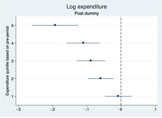
Figure 1 shows the effect on non-durable consumption expenditure⁴ by pre-demonetisation expenditure quintiles. Quintile 1 refers to the bottom 20% of households in the expenditure distribution (the poorest 20% of households), and quintile 5 refers to top 20% of households (the richest 20%). The horizontal or x-axis shows the log point⁵ change in non-durable consumption expenditure after demonetisation, with the corresponding 95% confidence intervals⁶. As we can see, the figure shows a decline of close to 20% for the richest households, while the effect is smaller for poorer households, and we cannot reject zero effect for the poorest households. In other words, the figure suggests that there seems to be no evidence of a decline in consumption of the poorest households, while we do see a decline in consumption for richer households.

Figure 1. Change in consumption expenditure by pre-demonetisation expenditure quintiles

How did the poor maintain their consumption?

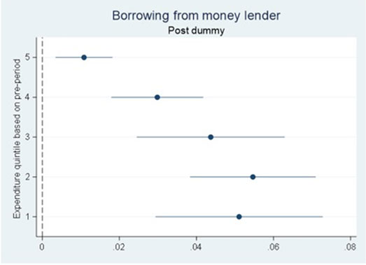
One question that arises from the above figure is: How did the poor maintain their consumption levels despite such a big shock? I find that the poor households relied a lot on informal credit, particularly from local moneylenders. Figure 2 shows the change in probability of having outstanding debt from moneylenders based on pre-demonetisation expenditure. We can see that the pattern in this figure is the opposite of the pattern in Figure 1. While the better-off show the maximum decline in consumption, they show the smallest increase (around 1 percentage point) in borrowing from moneylenders (the same result holds for any source of borrowing as well). The poorest households, on the other hand, show the largest increase (around 5 percentage points) in borrowing from moneylenders. The purposes data also show that the maximum increase in borrowing is for consumption. This result suggests that the poor used this credit to maintain their consumption.⁷

Figure 2. Borrowing from moneylender by pre-demonetisation expenditure quintiles

Why greater decline for the rich and not much for the poor

It is true that the poorer households had lower access to banking services which made them more reliant on cash as compared to the rich. But they also had lower consumption levels than the rich. And assuming diminishing marginal utility⁸, the loss in utility from a reduction in consumption at lower level would be much higher than the utility loss from the same reduction in consumption at higher levels. Therefore, the poor were willing to pay high transaction costs (for example, standing in lines for long hours) to get the required cash. Due to potential high cost of drop in consumption, they also had a higher incentive to use any consumption smoothing mechanism. The rich, on the other hand, could afford to reduce their consumption temporarily due to their high consumption levels. For example, if they bought their food products such as grains in bulk, they could afford not to buy goods in bulk in the months after demonetisation.

Relation between borrowing and cash reliance

To test if the increase in informal borrowing was higher for those households who rely more on cash, I focus on farmers and compare farmers who consume their own-grown food (subsistence farmers) to those who do not consume own-grown food (non-subsistence farmers). Focusing on farmers provides this natural categorisation of cash reliance. Farmers who consume their own food presumably deal less in cash as they need to do fewer purchases from the market. If the increase in borrowing is related to shortage of cash, then we should see that borrowing increases by more for non-subsistence farmers compared to subsistence farmers. This is exactly what I find in the data. Borrowing from moneylenders increases by 4 percentage points more for the non-subsistence farmers compared to subsistence farmers, suggesting that higher borrowing is related to more cash-reliance.

Caveat and implications

One caveat of the study is that due to data limitations, I do not observe interest payments the poor had to pay to maintain their consumption. The survey does not contain information about the amount of loan, or the interest rate paid; it only collects data on whether the household has any outstanding borrowing from a source or not. With this caveat, my results highlight the importance of informal networks in dealing with shocks in developing countries. My results also suggest that in the drive towards more formalisation, it is the informal sector which helped people in dealing with the shock, and this drive may have further strengthened some of the informal networks in the country.