Understanding the dynamics of the rupee-dollar exchange rate

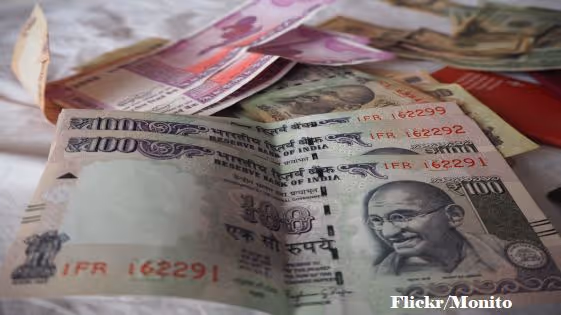
Since 1993, the Indian rupee (INR) has officially been following a market-determined exchange rate – price is determined by demand for and supply of foreign exchange – with intervention by the Reserve Bank of India from time-to-time. Analysing data from 2000-2020, Patnaik and Sengupta examine whether INR actually followed multiple exchange rate regimes, and if so, how the Central Bank managed exchange market pressure across these regimes.

In 1993, India officially moved towards a ‘market-determined exchange rate’ from a fixed peg to the US dollar (USD)¹. This was part of the liberalisation and deregulation reforms of the early 1990s. Since then, there has been a currency market, and according to the Reserve Bank of India (RBI) the Indian rupee (INR) has been following a market-determined exchange rate, implying that the price of the INR is determined by the demand for and supply of foreign exchange (forex). At the same time the RBI intervenes from time-to-time in the foreign exchange market to buy or sell dollars. The official stance has always been that the RBI does this in order to maintain “orderly conditions in the foreign exchange market” and to contain the volatility of INR. In a recent study (Patnaik and Sengupta 2021), we infer and document the evolution of India's exchange rate regime (ERR) from 2000 to 2020. We introduce a novel angle of analysing the ERR, by using an exchange market pressure index (EMP). Specifically, we examine whether INR followed multiple regimes in the last couple of decades despite being market-determined, and if so, how the exchange market pressure was managed by the RBI across the different exchange rate regimes.

The degree of foreign exchange intervention and the degree of flexibility in the exchange rates are likely to differ across the regimes based on the response of the RBI to the EMP. The de-jure classification of ERR of a country often diverges substantially from the de-facto ERR that exists in practice. Full information about the ERR is often not disclosed by central banks and hence, the ERR needs to be uncovered from historical data using statistical methods. Given the active foreign exchange intervention by the RBI, it is difficult to decipher India’s ERR by simply looking at the level of the exchange rate or the volatility. The actual rate that is observed is partly an outcome of the underlying macro-financial conditions or shocks faced by the economy, and partly of the intervention policy or currency policy of the central bank.

Exchange rate regimes

To estimate the various regimes that the INR might have experienced in the period from 2000 to 2020, we use a structural change methodology described in Zeileis et al. (2010). The essence of this methodology is that we estimate a ‘linear regression model’² using the returns on cross-currency exchange rates expressed in terms of a suitable ‘numeraire’ currency. We use the New Zealand dollar (NZD) as the numeraire currency, given its stability over a long period of time.

We then regress the INR on a basket of other currencies – USD, Euro, Japanese Yen (JPY) and British Pound (GBP) (all expressed in terms of the NZD) – in order to estimate the impact of these currencies on INR. These are the most important floating currencies in the world, that is, currencies which move in response to the forces of demand and supply in the forex market, and are not actively managed by the respective central banks. The regression, therefore, picks up the extent to which the INR/NZD rate fluctuates in response to fluctuations in any of the currencies.

For example, if INR is pegged to USD, then the corresponding estimated coefficient in the regression model will be close to one and all the other coefficients will be close to zero. If, on the other hand, INR is not pegged to any of these currencies, then all the coefficients will be different from zero and will reflect the true trade and financial linkages of the economy with the rest of the world. If INR is instead pegged to a basket of currencies, then the estimated coefficients would reflect the corresponding weights of the currencies in that basket. In the case of reduced exchange rate flexibility, the explanatory power of this regression (as seen from the ‘R-squared value’) would also be very high, while lower values would be obtained for floating currencies.

We then apply the Zeileis et al. (2010) structural change method, which helps us to uncover the breaks in the R-squared value as well as in the ‘error variance’ of this model. This gives us four exchange rate regimes in the case of INR. We show this in Figure 1 where the regimes are separated from each other by the dotted vertical lines. The figure plots the volatility of the INR-USD exchange rate across the four regimes. For each regime, we also mention the average volatility of the exchange rate at the top of the graph, to highlight the differences in the exchange rate flexibility across these periods.

Figure 1. Exchange rate regimes and volatility of INR/USD exchange rate

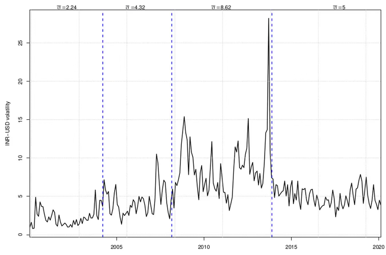
Source: BIS (Bank for International Settlements) database and authors’ calculations.

Notes: (i) This graph plots the annualised volatility of the INR/USD nominal exchange rate across the different exchange rate regimes. (ii) The average currency volatility in each regime is mentioned at the top of the graph.

Regime 1 (January 2000 to March 2004): The first regime can be categorised as one where INR was closely pegged to USD. The estimated coefficient of the USD is highly statistically significant and is close to 1 (0.95) while the coefficients of the remaining four currencies are close to zero. The R-squared value is also the highest among all regimes, further confirming a pegged ERR.
Regime 2 (March 2004 to February 2008): In the second regime the R-squared value comes down from 0.97 to 0.86. The INR seems to have shifted to a less tight peg where the weight of the USD, though still the highest, is lower than the first regime.
Regime 3 (March 2008 to November 2013): The next regime, in the aftermath of the Global Financial Crisis (GFC), is characterised by the lowest R-squared value. This can therefore be classified as the most flexible ERR in our sample period. The estimated coefficient of the USD is also the lowest implying much less weight assigned to USD in the basket of currencies.
Regime 4 (November 2013 to December 2020): The fourth and final regime lasts till the end of our sample period. It is the longest period under one single ERR. The flexibility of INR has reduced compared to the previous regime. The weight of USD is also the second highest in the sample period, implying that INR went back to being relatively more pegged to USD, compared to its increased flexibility in the preceding ERR.

RBI’s response to exchange market pressure

Once we have identified the regimes, we delve deeper into how the RBI managed the exchange rate across these regimes. For this purpose, we use an Exchange Market Pressure (EMP) index. EMP is the pressure that the exchange faces primarily owing to fluctuations in capital inflows and outflows. This pressure is resisted either through forex intervention (thereby causing a change in reserves), or relieved through a change in the exchange rate. While an analysis of the ERR focusses on observed changes in the currency, EMP allows us to understand how much of the observed change was policy-determined.

We use the EMP measure proposed by Patnaik et al. (2017) where the EMP is expressed in terms of a percentage change in the exchange rate over a one-month period. EMP is calculated as the actual change in the exchange rate that took place and the change that would have occurred in the absence of any forex intervention. A negative EMP value denotes an appreciation pressure vis-à-vis the USD, whereas a positive EMP value captures depreciation pressure.

In each of the four regimes of INR, we examine the proportion of EMP that was resisted through forex intervention by the RBI, and the proportion that was relieved through exchange rate change. To decipher this from the data, we plot the EMP series against the net spot market intervention³ in Figure 2.

Figure 2. Exchange market pressure and net spot market intervention

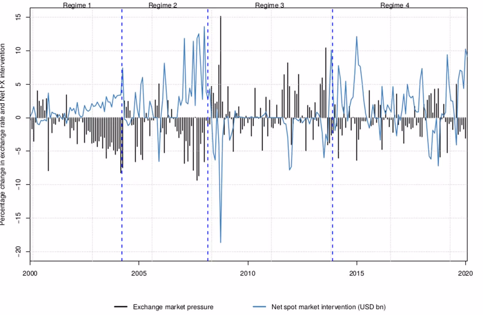
Source: BIS database and authors’ calculations.

Figure 2 shows us that during the first, second, and fourth exchange rate regimes, the EMP was mostly negative. This implies that the rupee experienced a pressure to appreciate for a majority of the sample period. The direction of the EMP changed around the time of the GFC. During the third ERR which ranges from 2008 to 2013, the rupee primarily faced a pressure to depreciate.

We also see that net spot market intervention was the lowest during the third regime and in the direction of net USD sales, whereas the higher forex interventions in the first, second, and fourth regimes were mostly in the direction of dollar purchases. Since the EMP by construction can be managed either through forex intervention or by letting the currency fluctuate, if we plotted the nominal INR--USD exchange rate instead of the net forex intervention in Figure 2, we would get an exact mirror image of the blue line in the graph.

In other words, in three out of the four regimes, the INR faced an appreciation pressure and the RBI intervened in the forex market to buy USD and reduce the extent of appreciation. In only one regime when INR faced a depreciation pressure (2008-2013), the RBI intervened relatively less in the forex market and did not sell a significant amount of USD from its forex reserves. During this period the exchange rate was predominantly in a floating regime, which truly responds to the market forces.

Asymmetric intervention by the RBI

It follows from the above discussion that while the RBI officially claims that it intervenes in the forex market with the objective of “ensuring orderly conditions in the foreign exchange market”, data show that this may not be the case.

In Figure 3, we plot the EMP measure against the RBI’s net foreign exchange intervention in a four-quadrant graph. The figure sheds some more light on the RBI’s asymmetric intervention in the currency market. For majority of the time period examined, the RBI has been a net buyer of USD in response to an appreciation pressure on INR, as seen from the density of the scatterplot in the lower right-hand quadrant of the graph.

Figure 3. RBI’s asymmetric intervention in the forex market

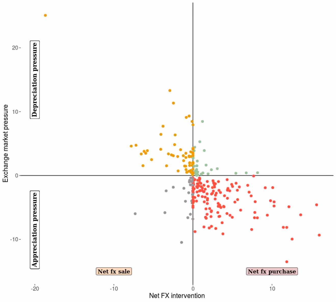
Source: RBI database and authors’ calculations.

Note: This is a four-quadrant graph plotting the monthly net forex intervention by the RBI against the EMP index.

This further suggests that the RBI does not intervene in the forex market only to contain volatility of INR because if that had indeed been the case, then there would have been a more well-rounded distribution of the scatterplot.

Conclusion

Using data-driven analysis, we find that INR has not consistently followed a market-determined exchange rate for most of the period between 2000 and 2020. The evolution of INR’s movement during this period can be described by four specific ERRs and only in one of these four regimes, the rupee came closest to being a flexible currency. This was the period from 2008 to 2013 in the aftermath of the GFC when the INR faced a pressure to depreciate and the RBI, instead of selling USD from its forex reserves to arrest the rupee movement, allowed the currency to depreciate. In all the other regimes, the RBI mostly bought USD in the forex market, thereby accumulating a large amount of reserves, with the attempt being to prevent INR from appreciating.

We find that when INR faces depreciation pressure, the RBI uses only a tiny fraction of reserves to defend the currency – the RBI is much more proactive in its currency management when INR faces pressure to appreciate. This indicates an inherent asymmetry in the RBI’s exchange rate management policy.

The authors thank Madhur Mehta, Prashant Parab and Surbhi Bhatia for their help with the data analysis and Josh Felman for his valuable suggestions.

I4I is now on Telegram. Please click here (@Ideas4India) to subscribe to our channel for quick updates on our content

Notes:

Prior to 1993, the exchange rate was determined with reference to the daily exchange rate movements of the USD and hence did not capture market dynamics.
Linear regression attempts to model the relationship between two variables by fitting a linear equation to observed data
Net intervention is defined as the total purchase of USD by the RBI in the forex market minus the total sale of USD.