Goods and services tax: Estimating optimal rates

Introduced in India in 2017, a key feature of the goods and services tax (GST) system is that the tax rate for a particular commodity is uniform across the country. Based on a counterfactual framework that incorporates regional diversity in prices and spending to estimate optimal commodity tax rates, this article argues for a departure from this universal GST practice in India.

In a landmark change to India’s fiscal system, the Good and Services Tax (GST) came into effect on 1 July 2017. Overhauling the existing system of indirect taxes, the GST replaced most indirect taxes, with the exception of a few state taxes.¹ The GST is imposed at every step in the production process, but is meant to be refunded to all parties in the various stages of production, other than the final consumer. It is a destination-based tax that is collected at the point of consumption, and not point of origin like previous taxes.

From a myriad of sales taxes, to GST

This feature of the GST is a significant departure from the previous system of indirect taxes in India, which involved the levy and collection of tax at different locations, as the item progressed through the production process. In a country of India’s geographical size and diversity, the production and distribution of an item is often spread across states and regions, separated by large distances. Pre-GST, this meant that the intermediate production process attracted taxes at different rates, payable to different tax collection agencies. Hence, the move to GST led to considerable simplification of the paperwork, and criticism of its implementation notwithstanding, it has been generally welcomed for this reason.

With the adoption of GST in 2017, India joined a select group of developing countries and emerging economies that follow this tax regime. India’s entry into the GST club is significant in view of its geographical and population size and its diversity of preferences. The GST has two features that have characterised the tax systems in the countries that have opted for it. First, GST rate is identical across the country² and, second, the tax rate is uniform across commodities. In adopting the GST, several countries have abandoned the second feature³ by exempting certain items. However, with the exception of India, the items that are not GST-exempt are generally taxed at a uniform rate. In India, in a further deviation from a strict adherence to the second feature, the basket of items is divided into five different tax slabs for tax collection: 0%, 5%, 12%, 18%, and 28%. However, the first feature was retained, namely that the tax rate on the same item is the same in all parts of the country.

Optimal commodity taxes

In a recent study (Majumder, Ray and Santra 2021), we examine GST rates in India by comparing them with our estimates of ‘counterfactual’ tax rates that are revenue-neutral with respect to the GST rates, that is, result in the same amount of tax revenue generation⁴. We focus on examining two features of GST in India’s federal setting: (i) identical tax rate for particular commodities across states, and (ii) uniform taxation of all commodities within a state. The counterfactual framework that we use to evaluate GST in the country is that of ‘optimal commodity taxes’ as distinct from indirect tax reform⁵. The former refers to designing a new tax system – as was the case with GST in India – with the focus of formulating a set of commodity tax rates that raises a pre-specified level of revenue while minimising the welfare loss due to taxation. On the other hand, the latter takes the existing tax system and seeks to enhance welfare, that is, to change the existing tax rates such that the current revenue is still raised but some are made better-off without making anyone worse-off. A cardinal principle underlying the theory of optimal commodity taxes is that these will depend crucially on prices and preferences (Ray 1986). In India, it is logical to expect optimal commodity taxes to vary across regions, in contrast to a conventional GST setting (Majumder, Ray and Sinha 2015). In what follows, we report evidence in favour of varying tax rates by region.

Spatial variation

The counterfactual tax rates are based on all-India data on private final consumption expenditure (PFCE) classified by items, obtained from the reports of the Ministry of Statistics and Programme Implementation. We consider overall PFCE and item-wise PFCE, at both current and constant prices⁶ for five broad item groups for the period between 1950-51 and 2017-18. These groups are: (i) Food and beverages, (ii) Clothing and footwear, (iii) Housing, water, electricity, gas, and other fuels, (iv) Health, education, transport, and communication, and (5) Miscellaneous. We compute item-specific consumer price indices (CPI) by taking a ratio of item-wise PFCEs at current and constant prices at the all-India level⁷.

We find that the estimated optimal commodity tax rates quite clearly bring out the required spatial variation in tax rates among Indian states. The variation is much less for housing and electricity, and health and education across states and across levels of ‘inequality aversion’ of the planner. This provides limited support to the principle of regional invariance of the tax rates underlying the first feature of the GST described above. We obtain ‘all-India’ optimal tax rates by treating the whole country as a single homogeneous entity – ignoring inter-state differences in preferences and prices, as is assumed by the first feature of the GST mentioned earlier. These calculations confirm that the all-India estimates hide large variation in optimal tax rates across states. In policy terms, the evidence is inconsistent with the regional invariance of the tax rates. The counterfactual evidence on commodity taxes also suggests that the current GST rates of 12%, 18% and 28% in the upper slabs find little support in the estimation of optimal commodity tax rates – the current GST rates are somewhat higher than is suggested by an application of ‘textbook’ principles.

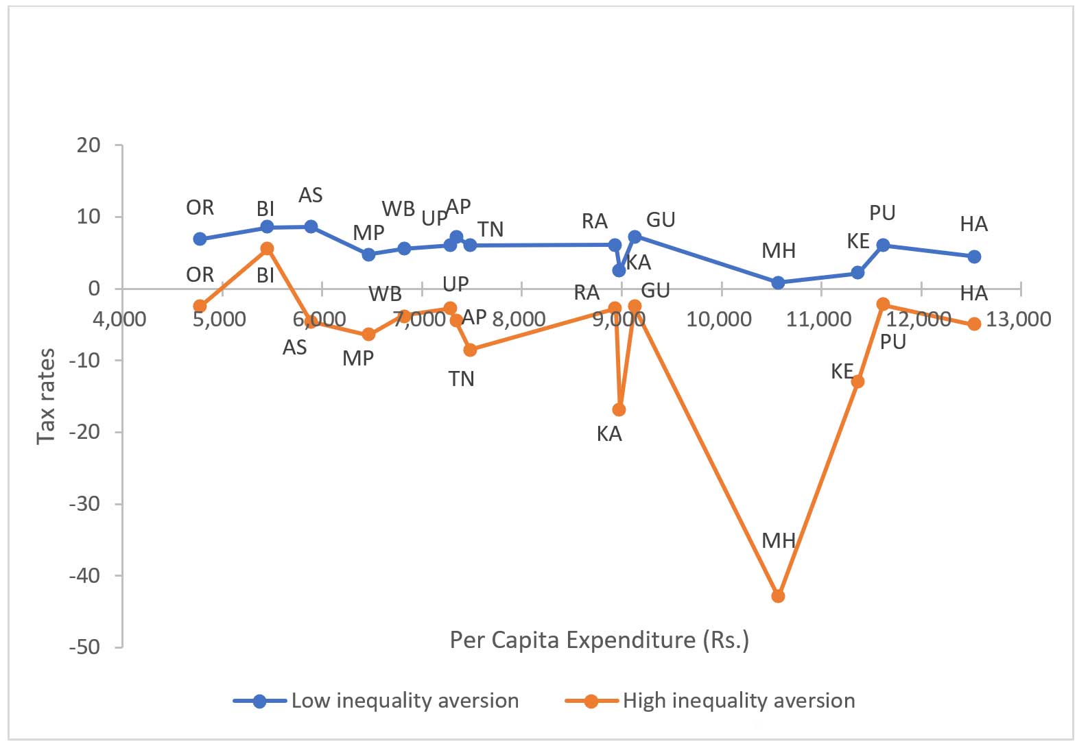
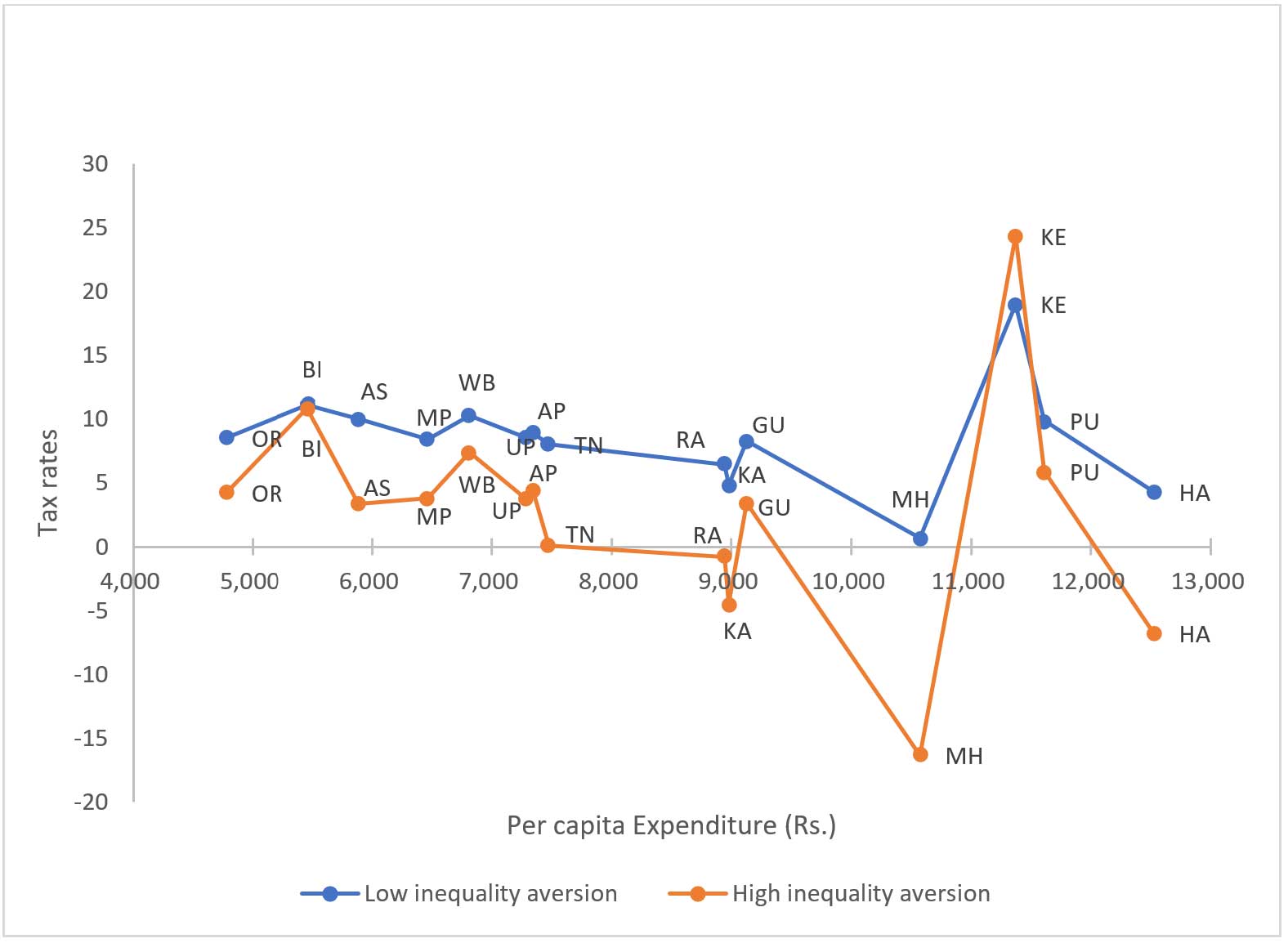
Figure 1 presents the optimal tax rates in each state plotted against the corresponding per capita total consumer expenditure of the states for different items for high and low inequality-aversion. We see that there is considerable spatial heterogeneity in the optimal commodity tax rates. Second, there is a strong negative association between the optimal tax rate of ‘food and beverages’ (necessity) and the state’s affluence as measured by its per capita expenditure, though less so for the other item of necessity, ‘clothing and footwear’. In other words, if states were allowed to levy different tax rates on the same item, provided these are all revenue-neutral, the more affluent states will tend to tax the two items of necessity at lower rates than the less affluent states. In contrast, for ‘housing, water, electricity, gas, and fuels’, this is not the case and there is a positive relationship with optimal tax rates as we move from poorer to richer states. Third, in case of both groups of necessities, namely, ‘food and beverages’ and ‘clothing and footwear’, the blue lines corresponding to the low inequality aversion lie above the orange lines that correspond to the higher level of inequality aversion – signifying lower tax and higher subsidy rates for these items with greater aversion to inequality.

Figure 1a. State-wise optimal tax/subsidy rates for ‘food and beverages’

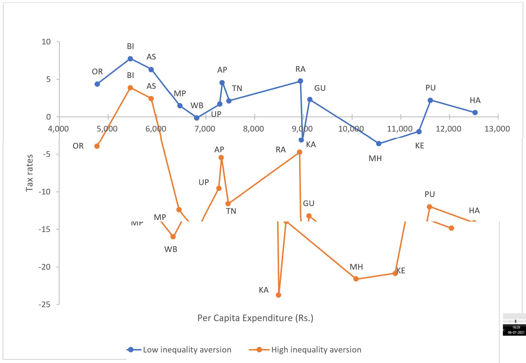
Note: A list of state abbreviations can be found here.

Figure 1b. State-wise optimal tax/subsidy rates for ‘clothing and footwear’

Since the tax rates must be revenue-neutral, it is worth noting that the position of the two lines gets reversed in the next two graphs corresponding to ‘housing, water, electricity, gas, and fuels’ and ‘health, education, transport and education’.

Figure 1c. State-wise optimal tax/subsidy rates for ‘housing, water, electricity, gas, and other fuels’

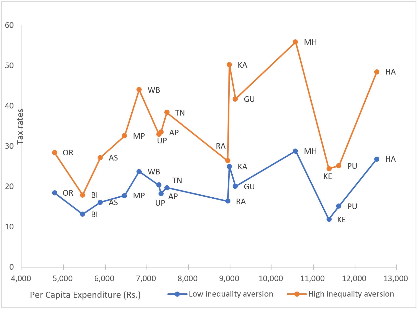
Figure 1d. State-wise optimal tax/subsidy rates for ‘health, education, transport, and communication’

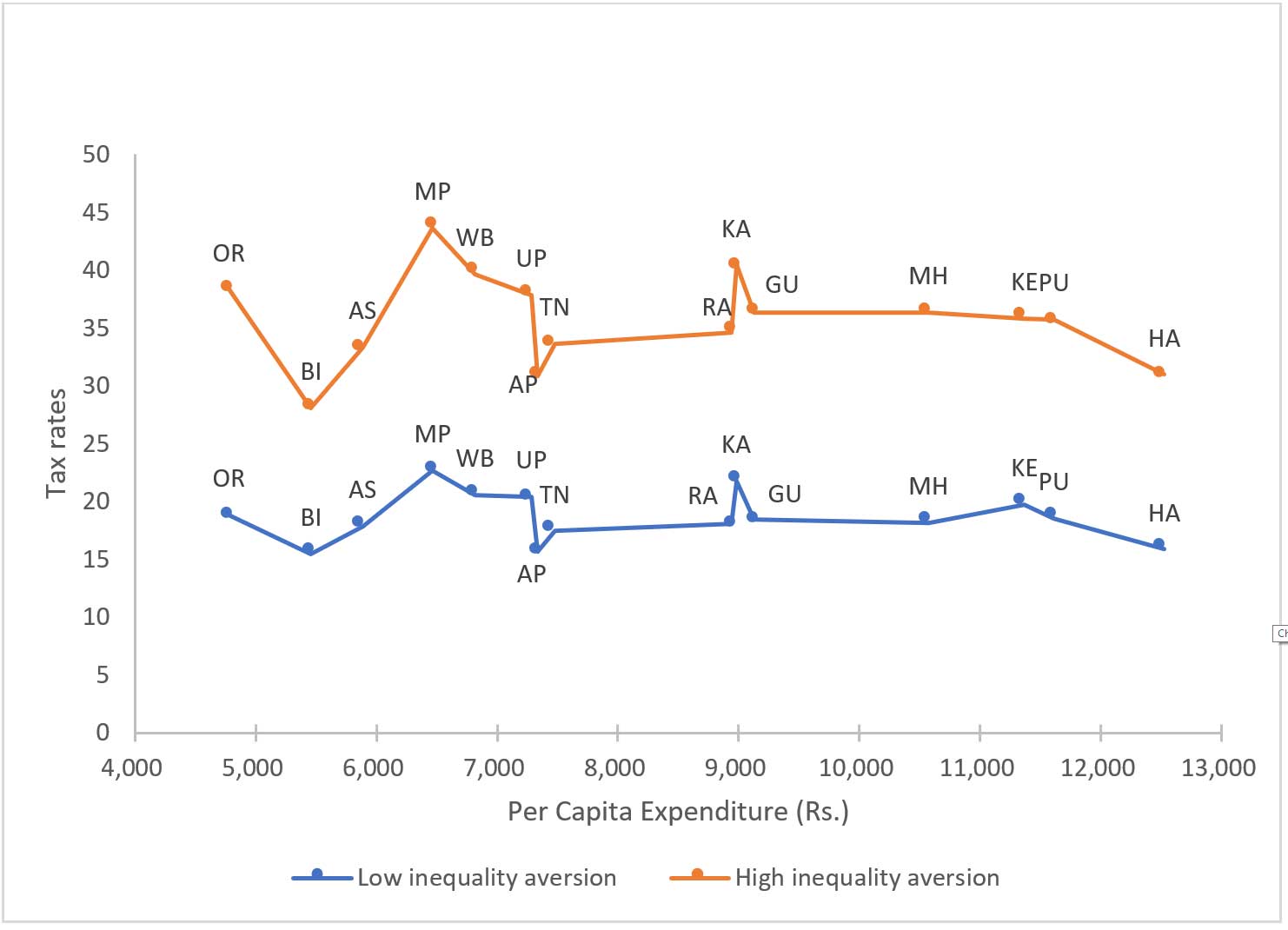
Figure 1e. State-wise optimal tax/subsidy rates for ‘miscellaneous items’

Policy implications

Our analysis has several implications for taxation policy in India. The findings suggest that uniform tax rates across states or commodities may not be ideal as there is wide variation in item-wise consumption patterns across states. If state-varying GST tax rates cannot be implemented, the tax rates arrived at centrally should be based on a population-share weighted average of the state-specific GST rates, taking account of diversity in regional prices and preferences. For this, centralised decision-making on GST rates by the nation-wide GST Council should be replaced by a decentralised system through the setting up of provincial GST councils that take account of regional preferences and prices. The provincial GST councils should then work in tandem to ensure tax coordination between the states, similar to that between countries in the EU.

I4I is now on Telegram. Please click here (@Ideas4India) to subscribe to our channel for quick updates on our content.

Notes:

For example, tax on items containing alcohol, tax on petroleum products, entertainment tax (levied by local bodies).
In several countries such as Canada, allowing the states or provinces to levy taxes in addition to the GST, implies that the commodity tax rate varies across regions.
In Australia, for example, GST exempts certain items such as basic food items, medical and healthcare services, but all the items on which the GST applies attract a tax rate of 10%. The same is true of Canada and New Zealand with a commodity invariant GST of 15% and 5%, respectively.
We find evidence of heterogeneity (across regions and across items) in the indirect tax settings in a federal context. We also present evidence on the tax progressivity of the counterfactual tax rates. For more details, see Majumder, Ray and Santra (2021).
Atkinson and Stiglitz (1980) contain a description of the former, Ahmad and Stern (1991) that of the latter, including application to Indian tax reform.
1999-2000 is taken as the base year for both overall and item-wise PFCE at constant prices, and item-specific CPI.
The price indices were converted to actual prices using a methodology proposed in Majumder, Ray and Santra (2021).