The per-capita state domestic product of Haryana (India’s richest state) was 5.6 times that of Bihar (poorest state) in 2017-18, up from 3.8 in 1996-97. Differences in urbanisation levels and inability of poorer regions to realise agglomeration benefits, are cited as reasons for the lack of convergence across states. Using 2018-19 Periodic Labour Force Survey data, this article examines spatial disparities in household earnings across the country.
Over the years, India has become more unequal. This is evident from the trends in the per-capita state domestic product (PCSDP) across its states. The tradition in the country is to benchmark the PCSDP of a state against that of Haryana – which has the highest PCSDP among large states. Consider the case of Bihar. Reserve Bank of India (RBI) data show that, the PCSDP of Haryana was 3.8 times that of Bihar (the poorest state) in 1996-97, and this increased to 5.6 times in 2017-18. The lack of convergence in PCSDP is also evident in data from consumption surveys conducted by India’s National Statistical Office. Poverty is concentrated in a handful of states (Naraparaju and Chandrasekhar 2021), and there has also been an increase in consumption inequality. Further, concerns have been expressed over the steady increase in the ratio of average urban to rural consumption over time (Datt et al. 2020).
Differences in the level of urbanisation at the sub-national level and the inability of poorer regions to realise the benefits from agglomerating economic activities, have been cited as reasons for the lack of convergence across states (Lamba and Subramanian 2020). Data from the 2011 Census indicate that the rate of urbanisation varies substantially within India – from just over 10% in the eastern state of Bihar, to over 45% in the southern state of Kerala.
Examining disparities in household earnings across states
In a recent study (Chandrasekhar et al. 2021), we examine the issue of spatial disparities in living standards across India using data from the Periodic Labour Force Survey (PLFS) (2018-19) of the National Statistical Office. As a welfare metric, we use monthly per capita household earnings (MPCHE), which is the ratio of total earnings of working members to total household members. These earnings can be by way of self-employment, salaried job, or casual work.
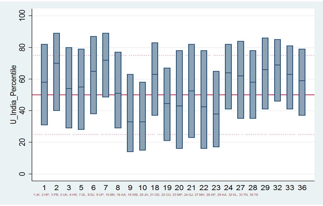
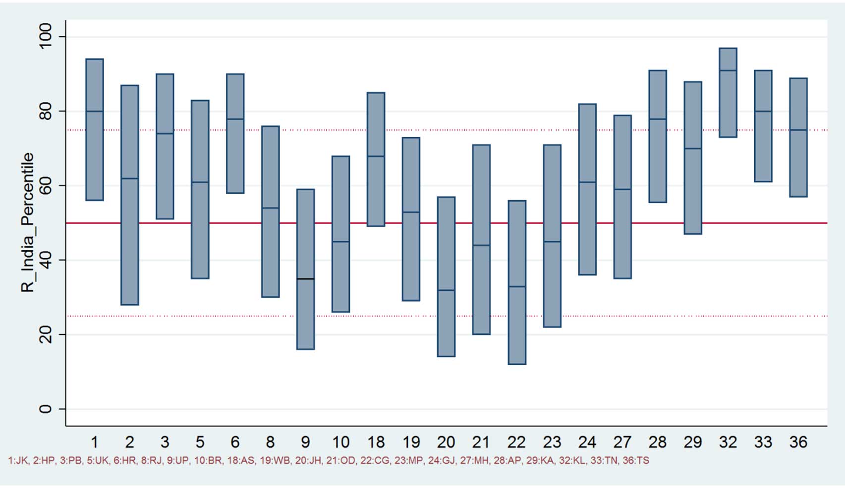
Figures 1a and 1b provide a visual description of differences in monthly per capita household earnings within India. The corresponding values in rupees are reported in Table 1.
Figure 1a. All-India distribution versus state-wise distribution of monthly per capita household earnings, rural India
Figure 1b. State-wise distribution versus all-India distribution of urban households, by MPCHE

Notes: (i) Authors’ calculations based on PLFS 2018-19 data. (ii) The vertical axis depicts the all-India distribution of MPCHE. (iii) The red dotted lines indicate the 25th, 50th and 75th percentile of the all-India distribution. (iv) The bars corresponding to each state identifies the position of the household in the state’s 25th, 50thand 75th percentile in the all-India distribution. (v) The state abbreviations used are as follows: 1: Jammu & Kashmir, 2: Himachal Pradesh, 3: Punjab, 5: Uttaranchal, 6: Haryana, 8: Rajasthan, 9: Uttar Pradesh, 10: Bihar, 18: Assam, 19: West Bengal, 20: Jharkhand, 21: Odisha, 22: Chhattisgarh, 23: Madhya Pradesh, 24: Gujarat, 27: Maharashtra, 28: Andhra Pradesh, 29: Karnataka, 32: Kerala, 33: Tamil Nadu, 36: Telangana.
Table 1. Cut-off values (in rupees) in all-India distribution of monthly per capita household earnings
|
Percentiles |
10th |
25th |
50th |
75th |
90th |
|
Rural |
1,125 |
1,600 |
2,425 |
3,750 |
5,625 |
|
Urban |
1,800 |
2,648 |
4,420 |
8,000 |
13,333 |
Consider Figure 1a. In both rural Kerala and Tamil Nadu, the household at the 25th percentile of the state's distribution has an MPCHE higher than the all-India median of Rs. 2,425. A few other states have a similar pattern. In fact, Kerala’s 25th percentile is nearly as high as the all-India 75th percentile (Rs. 3,750). In contrast in the states of Bihar and Uttar Pradesh, the median household has an MPCHE of Rs. 2,000 and Rs. 1,750, respectively – lower than the all-India median. In urban India, for a handful of states, the 25th percentile is below the-all India 25th percentile. In fact, when we rank states by median rural and urban MPCHE, the eight states with a concentration of India’s poor (in terms of consumption) are at the bottom of the ranking: Bihar, Chhattisgarh, Jharkhand, Madhya Pradesh, Odisha, Rajasthan, Uttar Pradesh, and West Bengal.
Interplay between urbanisation and inequality
While empirical literature on differences in living standards has sought to understand factors that would explain change in inequality over time (Kanbur and Zhuang 2013), we are interested in explaining differences in inequality across regions at a point in time. We focus on urbanisation as a key driver of these differences.
This interplay between urbanisation and inequality has traditionally been understood using ‘Kuznets’ process’ (Kuznets 1955). According to this framework, two things can be expected in the context of a poorer region with a low level of urbanisation. First, the difference between its rural and urban incomes should be lower vis-à-vis the richer and more urbanised regions. Second, the poorer regions should be less unequal.
We find that in Kerala, the ratio of average urban to rural MPCHE is the lowest at 1.23. This ratio is highest in Jharkhand (2.69), Odisha (2.81), and Chhattisgarh (3.01) – all much higher than the all-India figure (2.17). Hence, the first conjecture of the Kuznets’ process does not seem to hold. While it is true that in nearly all states, rural inequality is lower than urban inequality, there are other interesting patterns – it does not appear that all poor regions are characterised by lower inequality. Within the eight poorest states, inequality as measured by the Gini coefficient1, varies from 0.316 in Bihar to 0.476 in Chhattisgarh, while the estimate of the Gini coefficient is 0.378 in Tamil Nadu and 0.468 in Maharashtra. For India as a whole, Gini is estimated to be 0.446. We also provide corroboratory evidence that inequality hurts the poor – a one percentage point increase in Gini is associated with a 4.2% decrease in MPCHE for the bottom ventile2, on the contrary, a one percentage point increase in Gini is associated with a 3.1% increase in MPCHE in the top ventile.
In order to explain the difference in a state’s inequality in relation to the country as a whole, we adapt a decomposition method developed by Mookherjee and Shorrocks (1982) and quantify the relative importance of sectoral inequalities, urbanisation, and inter-sector income differences in explaining the variation in inequality across Indian states3. Using this decomposition, we show that high rural-urban income differences are largely responsible for high inequality in the states of Jharkhand, Odisha, and Chhattisgarh.
To illustrate the utility of this approach, consider the following – Bihar’s inequality is about 50% lower than all-India inequality, whereas Kerala’s is about 20% lower. Using this decomposition, we show that, almost 50% of Bihar’s low inequality is due to lower within-sector (in particular rural) inequality, whereas in Kerala, inequality is lower almost entirely due to lower rural-urban average MPCHE differences vis-à-vis all-India. On the other hand, Chhattisgarh’s inequality is about 13 percentage points higher than all-India, which is largely due to a high urban to rural average MPCHE ratio. In an accounting sense, all else being equal, if Chhattisgarh had the same urban-rural average MPCHE as all-India MPCHE, its inequality would have been lower by about 18% than its current level.
Concluding remarks
Recent news reports suggest that migrants who had returned to their villages due to the lockdown following the Covid-19 pandemic, have come back to the city because of lack of opportunities in their villages. This suggests that labour markets in the out-migration areas are unable to absorb the return migrants. This is not surprising in light of the evidence we provide of vast gulf in living standards between an out-migration state like Bihar and a relatively prosperous state like Tamil Nadu. To the extent that these migrants would have preferred to have remunerative job opportunities closer to home, our study underscores an urgent need for policymakers to focus on addressing India’s regional imbalances.
I4I is now on Telegram. Please click here (@Ideas4India) to subscribe to our channel for quick updates on our content
Notes:
- Gini coefficient is a measure of statistical dispersion, mainly used to enumerate income inequality. It is measured on a scale of 0 to 1; with 0 indicating perfect equality and 1 indicating maximal inequality.
- A ventile measure ranks and divides the dataset into 20 equal parts such that, if values of consumption are listed in ascending order, the bottom ventile would refer to the bottom 5% values in terms of consumption.
- For this exercise, we use mean log deviation as the measure of inequality.
Further Reading
- Chandrasekhar, S, K Naraparaju and A Sharma (2021), ‘Spatial disparities in household earnings in India: Role of urbanization, sectoral inequalities, and rural-urban differences’, IGIDR Working paper No. 2021-009.
- Datt, Gaurav, Martin Ravallion and Rinku Murgai (2020), “Poverty and Growth in India over six decades”, American Journal of Agricultural Economics, 102(1): 4-27.
- Kuznets, Simon (1955), “Economic Growth and Income Inequality”, The American Economic Review, 45(1): 1-28.
- Kanbur, Ravi and Juzhong Zhuang (2013), “Urbanization and Inequality in Asia”, Asian Development Review, 30(1):131-147. Available here.
- Lamba Rohit and Arvind Subramanian (2020), “Dynamism with Incommensurate Development: The Distinctive Indian Model”, Journal of Economic Perspectives, 34(1): 3-30.
- Mookherjee, Dilip and Anthony Shorrocks, “A Decomposition Analysis of the Trend in UK Income Inequality,” The Economic Journal, 92(368): 886-902.
- Naraparaju, K and S Chandrasekhar (2021), ‘Poverty Reduction in Rural India during 2004-05 to 2011-12: Role of Growth, Redistribution, and Population Shifts’, IGIDR Working paper No. 2021-015.


 18 August, 2021


Comments will be held for moderation. Your contact information will not be made public.