The Central Statistics Office recently changed the way GDP is calculated in India, revising the growth estimate for 2013-14 from 4.7% to 6.9%. Many are confused and skeptical about the new numbers, partly owing to a perceived mismatch between the higher growth and underperformance of other economic indicators. In this article, Saugata Bhattacharya, Senior Vice President and Chief Economist at Axis Bank, contends that a credible economic rationale underlines the new methodology. He demonstrates that corporate data are consistent with the national accounts estimates, and this has a bearing on future growth expectations.

It is clear from news articles and commentaries that there is not just significant confusion about interpreting the new 2011-12 based GDP (gross domestic product) series, but fairly deep skepticism about their representation of underlying economic trends. This skepticism arises predominantly from the conflicting perceptions of the relatively high GDP growth versus the underperformance of other high-frequency indicators like the Index of Industrial Production (IIP), freight movement, excise tax collections (net of petroleum products) and so on. In particular, the low credit offtake from banks is emphasised as being inconsistent with the financing needs presumed required for this high GDP growth.

The puzzle of the new GDP series

This is a variant of the classic Sherlock Holmes query: why did the dog not bark in the night? The puzzle of the new GDP numbers, in other words, is as follows. The methodology uses the United Nations System of National Accounts 2008 (SNA), consistent with global usage. Moreover, the database used for the value added extrapolations is the Ministry of Corporate Affairs MCA21 database, containing accounts of over 400,000 companies. In contrast, the preliminary estimates of the old GDP series were derived from a database of less than 5,000 companies (sourced from the Reserve Bank of India (RBI)). Using a standardised methodology operating on a vastly superior database, how did the revision result in this extent of skepticism and puzzlement?

We have been able to reconcile a fair part of this perceived discrepancy. The fundamental change was a re-orientation from our “volume” mindset into a “value” one; things then begin to fall in place. Note, too, that to make sense of this national accounts ecosystem, the entire value chain of the GDP from output (sales) to profits, its deployment for capex (capital expenditure) and investment, funding via savings, dividend payouts and their effects on consumption and its feedback into the GDP loop needs to be considered. Our dataset for our attempt to validate the GDP estimates is aggregated from 4,500 companies (sourced from the CMIE (Centre for Monitoring Indian Economy Pvt. Ltd.) Prowess database)¹ .

Let me emphasise once more that this is not an attempt to explain the technical details underlying the SNA 2008 methodology, although we would certainly be able to add colour to our reconciliation if we were to drill down into sector assumptions and estimations underlying the GDP numbers.

First, a little background on the new GDP. The nominal levels of the GDP started out lower in FY12 (Financial Year 2011-12) compared to the old levels and then climbed back up to the previous levels by FY14, thereby showing higher rates of nominal growth than the old series (Figure 1).

Figure1. Nominal GDP as per old and new series

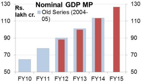Note: MP denotes market prices.

At the same time, real value added growth in the new GDP series has also been higher than in the older series for the respective years (Figure 2).

Figure 2. Real GDP and real Gross Value Added a per old and new series

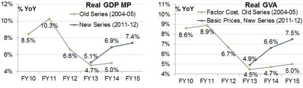
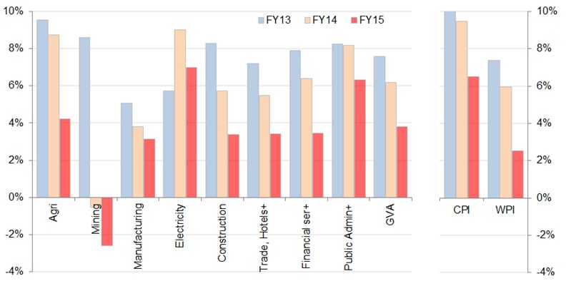
One reason for the higher real growth in the new GDP was a boost from the GDP deflators which have been lower than the CPI (Consumer Price Index) inflation numbers of the respective years (Figure 3)². This makes sense since the GDP deflators are a mix of WPI (Wholesale Price Index) and CPI metrics and some others which are implied deflators. Moreover, the use of WPI metrics has increased in the structure of the deflators, since these are largely used for the manufacturing segment, the share of which is now higher in the GDP, being based on “enterprise” rather than “establishment” accounting³ . In addition, the new 2012 base CPI had led to slight drop in inflation compared to the previous series. Although this is only a heuristic explanation, note that overall GVA (Gross Value Added) inflation has been falling during the three years for which GDP growth is reported; for the sale level of nominal growth, real GDP growth would have been higher.

Figure 3. Comparison of inflation derived from GDP Deflators with Consumer and Wholesale Price Indices

Mapping metrics from corporate financial accounts to national accounts

The core part of the process of reconciliation is to choose and then map the appropriate metrics from corporate financial accounts, which are likely to be the closest proxies to the key value added constructs in national accounts. This is important since many of us understand corporate accounts more instinctively and intuitively than GDP methods. In corporate finance terms, the Value Added component of nominal GDP is closely approximated by the sum of operating profits (Profits Before Depreciation, Interest and Taxes (PBDIT)) and compensation to employees (salaries and wages). If one tracks the two quantities over the two years (FY13 and FY14) for which corresponding data is available (FY15 corporate data is still sketchy), one can clearly see the co-movement of these metrics. This co-movement becomes even more pronounced if one tracks the two metrics on a quarterly basis (Figure 4). This correspondence is likely to be even sharper if we exclude the agriculture segment of GDP Value Added, since this sector will have a relatively small overlap with the reported corporate results.

Figure 4. Comparison of growth statistics of GDP and corporate results

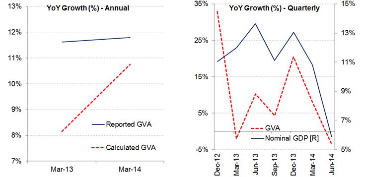Notes: (i) For annual data, meaningful comparisons are available only for two years (FY13 and FY14), since only a small set of (non-financial) companies have declared their annual reports as of now. (ii) YoY stands for Year-on-Year.

The next logical question is whether the large proportion of “small” companies in the MCA21 database might have something to do with the perceived disconnect between the new and old GDP series. In other words, might smaller companies (whose accounts were not available in the smaller dataset used for the old series) have grown sufficiently fast to have provided the boost to overall GDP growth in the new series? We have little idea of the structure of the MCA21 data. But we can perform an experiment, limited in scope, with the 4500 odd companies whose information we do have. If we quartile these companies in terms of their turnover, generally, larger companies have done better both on sales and profits (Figure 5). So we presume that this holds true for even the MCA21 dataset, and is not a major contributor of the reported high growth, although we are led to believe that smaller companies might have had a significant contribution to growth in FY13.

Figure 5. Trends in key operating parameters of companies classified by sales (turnover) size

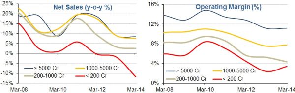
Figure 6. Savings rates of economic groups (as % of GDP)

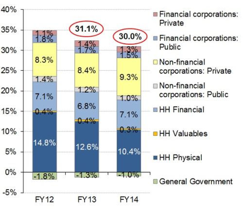
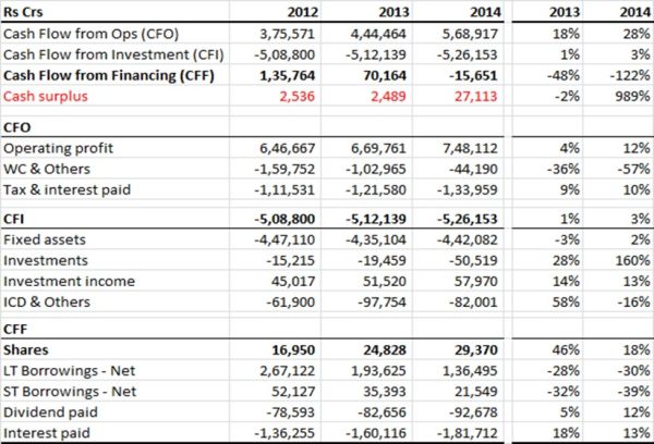
The next issue is the use of these financial savings. Remember the doubt about the compatibility of high GDP growth and low credit offtake? One hypothesis is that companies over the past few years have used their profits (internal accruals) to fund at least a part of their lower capex requirements. The sample of 4,500 companies which we have used reported a rise in Cash Flow from Operations from Rs 3.75 trillion in FY12 to Rs 5.69 trn in FY14 (Table 1). In turn, investment in fixed assets remained stable at around Rs 4.4 trn during all three years. At the same time, long- and short-term borrowings (from banks and other intermediaries) have fallen from about Rs 3.2 trillion in FY12 to about Rs 1.6 trn in FY14), highlighting both the slowing demand for funds for additional capex and the falling reliance on external credit sources.

Table 1. Summary of earnings and deployment of funds in the corporate sector

Note: Positive numbers are inflow for corporates, negative are outflows.

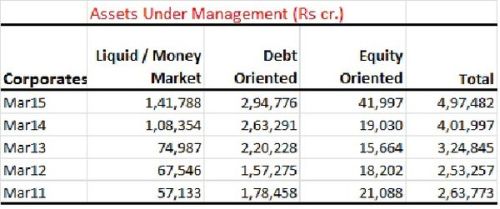
Coterminous to the build-up of cash flows of companies, investments in financial assets rose from Rs. 150 bn to Rs. 505 bn over the three years. (FY12–FY14) A large part of these investments by corporates in financial products shows up in the Assets Under Management (AUMs) of Mutual Funds (MFs). Corporate investments in MFs rose from Rs. 2.5 trn at end-March 2012 to Rs. 4 trn at end-March 20114 and thereafter to almost Rs. 5 trn in FY15. Incidentally, retail investments increased much more modestly from FY12 to FY14, but jumped sharply thereafter in FY15, both due to the rise in share indices and at least partially due to the increased dividend payouts by corporates. MF’s in turn invested heavily in debt-oriented and money market funds, presumably in expectations of a falling interest rate environment (Table 2). However, the deployment and flow of funds from MFs into specific end-uses needs to be understood in more detail.

Table 2. Corporate contributions to Assets Under Management of Mutual Funds

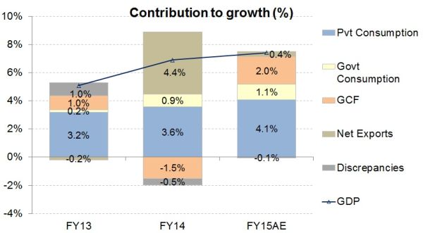
Given the large deployments in debt-oriented MFs, the latter have presumably contributed significantly to funding the Union and state governments’ borrowing programmes (and expenditure). How this is likely to have fed back into the GDP with a lag is mostly in the realm of speculation, not even hypotheses. The dynamics of transfer between the various components of GDP is too complex to be investigated at any length here. Figure 7 indicates how the higher government expenditures, primarily revenue spending, might have contributed to the private consumption in GDP. Government expenditures, particularly capital expenditures, had been drawn down sharply in FY14, and this is likely to have contributed to the shrinking of Gross Capital Formation in that year.

Figure 7. Decomposition of GDP growth contributions into demand components

What this means for India’s growth rates

The most important takeaway from this interpretation is as follows: Value added has been the source of the high GDP growth over the past three years, with falling commodities prices and cost-rationalisation driven efficiency gains the main drivers; this now might be coming to an end. In the near term, till growth (and corporate pricing power) increases, GDP growth might start reverting to the volume-oriented growth we analysts are more comfortable with. In other words, FY16 growth might not be much higher than the estimated 7.3% GDP growth in FY15.

Views are personal. Sanket Tandon and Abhay More contributed to the article.
A shorter version of this article appeared on the Economic Times Blog.

Notes:

1. The set of companies in this dataset are selected based on the availability and consistency of their reporting since FY12.
2. Real GDP growth is nominal GDP growth minus deflator-based inflation.
3. The establishment approach involves calculating production plant by plant. On the other hand, in the enterprise approach, the activities at headquarters are taken into account. For instance, the latter includes the various marketing and sales promotion efforts that are undertaken at the headquarter level after an item has been produced.