

 03 March, 2023


There is a growing literature on intergenerational educational mobility that explores how parental education influences the educational attainment of children. This article compares three empirical models widely used to study intergenerational educational mobility. Using data from India, China and Indonesia, it finds that conclusions regarding educational mobility vary substantially across different models. It argues that rank-based measures are not suitable for understanding the effects of economic policy, and suggests that policy advice should focus on the measures based on years of schooling.
Education is widely considered to be a key to escape poverty and achieve economic and social success, especially for the children born into disadvantaged households (Sen 1999, Rajan 2010, Stiglitz 2012). Whether children from disadvantaged background are left behind in an increasingly skill-intensive economy is an important question for policymakers. To explore this question, a growing literature on intergenerational educational mobility (IEM) studies how parental education influences educational attainment of children. The fundamental argument, developed by Roemer (1998), is that children should not be held responsible for the “circumstances” inherited at birth, with parental education being a salient inherited circumstance. If the link between parental education and children’s education is strong, it implies low mobility, as children’s own effort and choices play a minor role in their educational outcomes.
Understanding intergenerational educational mobility: Conceptual Issues
The empirical models widely used in the current literature on IEM depend on one of three units of measurement for educational attainment:
- Years of schooling
- Years of schooling, normalised by its standard deviation1 for each generation
- Rank in schooling distribution of each generation
Once an indicator of educational attainment is chosen, a linear mobility equation is estimated by regressing children’s education on parent’s education, and the slope parameter is a measure of ‘intergenerational persistence’2 Higher persistence implies lower relative mobility because children’s education is strongly tied down to that of parents. In linear models, the slope of the regression for years of schooling is called intergenerational regression coefficient (IGRC, for short) and the slope of the normalized years of schooling regression is known as intergenerational correlation (IGC, for short). Following the influential work of Chetty et al. (2014) on income mobility in USA, some recent studies of IEM have adopted rank in schooling3 distribution in a generation as the preferred indicator of educational attainment.
While one or more of these measures are frequently used in various studies, a systematic comparative analysis of all three measures is lacking in the literature. In a recent study (Ahsan et al. 2022), we aim to fill this gap. We explore theoretical and empirical differences among these three measures which may lead to conflicting conclusions. This provides guidance for researchers and policy analysts who may be confronted with such conflicts.
Our study
We use exceptionally rich data from three large countries – China Family Panel Studies (2010) for China, India Human Development Survey (2012) for India, and Indonesian Family Life Survey (2014) for Indonesia. These data sets are especially suited for intergenerational mobility analysis as they include information on non-resident children – children no longer residing with their parents– and thus do not suffer from sample truncation4.
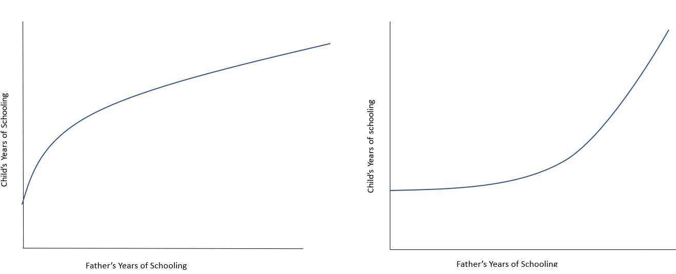
In Ahsan et al. (2022), we estimate both linear and quadratic mobility equations5. Linearity is an untested assumption in most existing studies. However, recent theory (Becker et al. 2015, 2018) suggests that a mobility equation can be either concave or convex6 depending on the net effect of two opposing forces: i) diminishing returns to financial investment, and ii) complementarity between financial investment and parental education. When such complementarity is stronger or weaker than the diminishing returns, it leads to a convex and concave mobility equation respectively (see Figure 1). Our estimates suggest that the mobility curve is convex in rural Indonesia and urban China, but concave in both rural and urban areas in India. This implies that the educational opportunities faced by children of uneducated fathers in India are very limited.
Figure 1: A concave (left) and convex (right) intergenerational educational mobility curve
To Normalise or not to normalise
As noted earlier, relative mobility7 is measured by the slope of the mobility equation. In a linear model, the slope is called Intergenerational Regression Coefficient (IGRC) for years of schooling, and Intergenerational Correlation (IGC) for normalised schooling. Some authors (see, for example, Hertz et al. 2008), argue that IGC is preferable because it neutralises the changing inequality across generations by making variances equal to 1. While the mobility equation for IGRC is derived from a Becker-Tomes model, there is no clear theoretical foundation for the mobility equation for IGC in the existing literature. We developed a simple approach that interprets the IGC estimates in terms of the Becker-Tomes model and inequality of opportunity perspective of Roemer (1998).8
It has been noted by some authors that IGRC and IGC often give different conclusions. While IGRC estimates suggest secular improvements in relative educational mobility, the IGC estimates show no such improvements (Hertz et al. 2008, Neidhofer et al. 2018). It is not clear how to interpret such conflicting evidence beyond simply observing that the two measures use different units. In our study, we provide an explanation by demonstrating that the elasticity of IGC with respect to IGRC is always less than 1, which implies much less variation in IGC. This result is also important for policy evaluation because IGC is less sensitive to policy changes and thus may fail to detect the impact of policies on relative educational mobility. This is because it is partly determined by factors unrelated to family background such as children’s own effort level, and exogeneous health and educational shocks to a child.
We find important differences in IGRC and IGC estimates between rural and urban households and across birth cohorts. For example, according to the IGRC estimates in India, rural households have less relative mobility than urban households. In contrast, the IGC estimates for rural and urban India suggest a higher relative mobility in rural India! Exploiting the theoretical link between IGC and IGRC, we show that this reversal is caused by two factors: (i) a higher cross-sectional inequality among urban parents, and (ii) a lower idiosyncratic component of children’s schooling variance capturing their own effort and choices (for more detail, refer to Ahsan et al. (2022)). Our approach is useful for understanding the mechanisms behind such measurement conflicts in other countries.
Challenges in interpreting rank-based measures of IEM
Rank-based analysis of IEM has been gaining popularity in recent years (see, for example, Andrade and Thomsen (2018) on Denmark and USA, Hilger (2015) on USA, Neidhofer et al. (2018) on Latin America, Asher et al. (forthcoming) on India, and Chen et al. (2015) on China). The current literature, however, largely ignores the implications of the fact that, unlike income, years of schooling is a discrete variable – which is to say that the maximum schooling one can attain is a PhD, but there is no maximum limit to how rich one can be. In Ahsan et al. (2022), we point out that percentile ranks remove such growth in income at the top of the distribution, but for education, such concerns are simply irrelevant. Additionally, ranks calculated from schooling distribution (mid-rank method) of each generation often fail to equalise the variances (inequality) across generations9. The argument that rank-based approach is preferable because it neutralises changing inequality and growth effects is valid for income (Chetty et al. 2014), but not for education. IGC is preferable to the rank-based measure of relative educational mobility on two counts: IGC makes inequality across generations equal, and the estimate can be interpreted in terms of the Becker-Tomes model. As noted by Heckman (2016), it is difficult to interpret the rank-based measures within the Becker-Tomes framework.
We find that evidence from the rank-based linear model yields different conclusions: the measure of educational mobility in rural India is lower than in urban India, but the reverse is true for IGRC estimate based on years of schooling. However, the linear rank-based model is rejected in all three countries that we analyse. This is different from the evidence of linearity for income ranks in the USA reported by Chetty et al. (2014). Rank transformation consistently makes the mobility equation more convex (or less concave), which mechanically generates higher relative mobility for the uneducated households. The shape of the mobility curve based on ranks may even be fundamentally different – the mobility curve in India is concave for both years of schooling and normalised years of schooling, but convex for ranks!
Overall, the rank-based approach yields substantially different results compared to the other two approaches. This suggests that rank-based measures capture very different mechanisms. A large and mature literature in sociology emphasises that the rank-based measures are likely to primarily capture the effects of formal and informal institutions (rules of the game) rather than the effects of economic policy and structural change captured by IGRC and IGC (Torche 2013). For example, a substantial change in the caste system, or gender norms in a patrilineal state in India would affect the rank-based measures much more than a change in economic policy such as trade liberalisation or expansion of private schools in rural areas.
Policy advice
The above discussion raises an important question: how do we advise policymakers when different models of mobility give conflicting conclusions about a policy? In Ahsan et al. (2023), we report such a conflict: conclusions about the impact of INPRES primary schools in Indonesia (where 61,000 schools were constructed in the early 1970s) on relative educational mobility of children are dramatically different when a rank-based model is used. The school expansion reduced IGRC and IGC, especially for the sons born to uneducated fathers, but the policy was completely ineffective according to the rank-based measure.
The inequality of opportunity perspective of Roemer (1998) suggests a simple approach to policy evaluation for IEM. A policy can be considered effective if it weakens the influence of circumstances inherited by birth on children’s educational attainment. Since parental education is a salient circumstance inherited by children, testing policy effectiveness is equivalent to testing whether a policy reduces IGRC. From this perspective, school construction was effective in improving relative mobility in Indonesia because it reduced IGRC, even though it failed to change the underlying institutional matrix captured by the rank-based measure of relative mobility (IRRS).
The broader lesson here is that when evaluating the effects of a policy on relative educational mobility, it is unwise to rely on rank-based measures exclusively. This is of wider relevance, as recent studies on intergenerational educational mobility in developing countries are increasingly abandoning IGRC and IGC in favor of the rank-based model.
Notes:
- Standard deviation is a measure used to quantify the amount of dispersion in a sample of values (in this case, years of schooling) from the mean value of that sample.
- The slope of a regression line is the change in the dependent variable in response to a unit increase in the independent variable. The slope of the mobility equation measures the change in children’s educational attainment for every additional year of their parent’s education.
- This distribution uses percentile ranks, calculated from the years of schooling data for parents and children separately. The slope of the rank-rank linear regression is called intergenerational rank-rank slope (IRRS, for short).
- Sample truncation is when some observations from a sample are systematically excluded from a household survey. Recent evidence suggests that co-resident samples lead to substantial downward bias in the estimate of relative mobility (Emran et al. 2018).
- A linear equation is one with variables that have no power higher than 1; a linear equation produces a straight line when graphed, while quadratic equation produces a parabola.
- The equilibrium relationship between parents’ and children’s education may be convex or concave. Convexity results in especially high levels of intergenerational persistence in educated households, as successive generations of educated families do not regress toward the population mean. In a concave function, although parental human capital raises the productivity of investments in children’s human capital, successive generations regress toward the population mean. As a result, children born in uneducated families find it difficult to attain higher education.
- Relative mobility answers the question of how many years of schooling a child expects to gain on average for every one additional year of schooling their father or mother has attained.
- The Becker-Tomes model derives a mobility curve based on parents’ optimal investments in children’s education where credit market access plays a central role. The ability of a parent to invest depends on their wealth, because the poor cannot borrow from the banks to finance children’s education. The inequality of opportunity (IOP) is a theory of distributive justice developed by Roemer (1998). The fundamental premise of IOP is that children’s economic and social success should depend only on their effort and choices, not on their family background, because the family a child is born into is not chosen by the child.
- The mid rank method assigns the midpoint value to the observations bunched at a given level of schooling. For example, if 20% of fathers have zero schooling, then they are assigned a rank of 10th percentile.
Further Reading
- Ahsan, MN, MS Emran, H Jiang, O Murphy and F Shilpi (2022), ‘When Measures Conflict: Towards a Better Understanding of Intergenerational Educational Mobility’, SSRN Paper.
- Ahsan, MN, F Shilpi and M. Shahe Emran (2023), ‘Public Primary School Expansion, Gender-Based Crowding Out, and Intergenerational Educational Mobility’, Working Paper. Available here.
- Andrade, Stefan B and Jens-Peter Thomsen (2018), “Intergenerational educational mobility in Denmark and the United States”, Sociological Science,5: 93-113.
- Asher, S, P Novosad and C Rifkin (forthcoming), “Intergenerational Mobility in India: Estimates from New Methods and Administrative Data”, American Economic Journal: Applied Economics, forthcoming.
- Becker, Gary S, Scott Duke Kominers, Kevin M Murphy and Jörg L Spenkuch (2018), “A theory of intergenerational mobility”, Journal of Political Economy, 126(S1): S7-S25.
- Becker, G, Kominers, SD, Murphy, K, and Spenkuch, J (2015), ‘A Theory of Intergenerational Mobility’, MPRA Paper 66334, University Library of Munich.
- Chen, Yuyu, Suresh Naidu, Tinghua Yu and Noam Yuchtman (2015), “Intergenerational mobility and institutional change in 20th century China”, Explorations in Economic History, 58: 44-73. Available here.
- Chetty, Raj, Nathaniel Hendren, Patrick Kline and Emmanuel Saez (2014), “Where is the land of opportunity? The geography of intergenerational mobility in the United States”, The Quarterly Journal of Economics, 129(4): 1553-1623.
- Deutscher, Nathan and Bhashkar Mazumder (2023). “Measuring Intergenerational Income Mobility: A Synthesis of Approaches”, Journal of Economic Literature, forthcoming.
- Emran, M Shahe, William Greene and Forhad Shilpi (2018), “When measure matters coresidency, truncation bias, and intergenerational mobility in developing countries”, Journal of Human Resources,53(3): 589-607.
- Heckman, J. (2016), ‘The Economics of Family Influence and Inequality’, ASSA Course Lecture on Microeconomics of Life Course Inequality, University of Chicago.
- Hertz, Thomas, Tamara Jayasundera, Patrizio Piraino, Sibel Selcuk, Nicole Smith and Alina Verashchagina (2008), “The Inheritance of Educational Inequality: International Comparisons and Fifty-Year Trends”, Advances in Economic Analysis & Policy, 7(2).
- Hilger, NG (2015), ‘The Great Escape: Intergenerational Mobility in the United States Since 1940’, NBER Working Paper 21217.
- Neidhofer, Guido, Joaquin Serrano and Leonardo Gasparini (2018), “Educational Inequality and Intergenerational Mobility in Latin America: A New Database”, Journal of Development Economics, 134(C): 329-49.
- Rajan, R (2010), Fault Lines: How Hidden Fractures Still Threaten the World Economy, Princeton University Press, Princeton.
- Roemer, JE (1994), Equality of Opportunity, Harvard University Press.
- Sen, AK (1999), Development as Freedom, Oxford University Press, Oxford.
- Stiglitz, JE (2012), The Price of Inequality, W.W. Norton, New York.
- Torche, F (2013), ‘How do we characteristically measure and analyze intergenerational mobility?’, Working Paper, Stanford Center on Poverty and Inequality.

Comments will be held for moderation. Your contact information will not be made public.