

 10 April, 2023


Attempts have been made to estimate poverty in India with biased survey data, by adjusting household weights to remove the bias. Based on simulation exercises with artificially contaminated household surveys, Drèze and Somanchi illustrate the limitations of this method. Its ability to correct poverty estimates varies wildly, depending on the nature of the underlying bias, which may be hard to guess – there lies the rub. When the bias changes over time, estimating poverty trends becomes truly problematic.
Poverty estimation in India has traditionally relied on consumption expenditure surveys (CES) to estimate the share of the population whose per capita expenditure lies below the ‘poverty line’. Until recently, CES rounds were conducted at regular intervals by the National Sample Survey Organisation (now National Statistical Office). With the suppression of the 2017-18 round by the central government, however, the last available CES round (2011-12) is now more than a decade old. This has thrown a shroud of darkness on poverty levels and trends.
Meanwhile, the Centre for Monitoring Indian Economy (CMIE) launched a series of large-scale Consumer Pyramid Household Surveys (CPHS) that include consumer expenditure data. In principle, CPHS data could be used for poverty estimation. Unfortunately, the CPHS surveys fail basic tests of national representativeness (Drèze and Somanchi 2021, Somanchi 2021). In particular, poor households seem to be underrepresented in these surveys. The bias is far from trivial: according to CPHS, for instance, 100% of households in Bihar (India’s poorest state) had water within the premises, 98% had a toilet within the house and 95% had a television in 2019 – this is poetry. The corresponding figures from the fifth National Family Health Survey (NFHS), a fairly reliable source, are much lower as one would expect: 89%, 62% and 35% respectively.1 There are major biases at the national level, too: for instance, the share of adults with no formal education in late 2018 was just 2% according to CPHS, compared with 17% according to the Periodic Labour Force Survey (PLFS).
Acknowledging these biases, two World Bank economists recently proposed an interesting method to correct them (Roy and van der Weide 2022, hereafter RW).2 Their study covers a lot of ground, but we focus on the correction method for now. This method consists of “re-weighting” the CPHS observations in a way that brings the means of basic socioeconomic variables in line with independent, credible estimates of these statistics – for instance, education levels. The re-weighting technique, discussed below, builds on the notion of “maximum entropy” (max-entropy for short). RW’s poverty estimates based on re-weighted CPHS data are now the official World Bank poverty estimates for India in recent years (Aguilar et al. 2022, World Bank 2022).
RW’s method is certainly a step outward from the black hole. But how well does it work? We try to shed some light on this using Monte Carlo simulations. Briefly, we create an artificial under-representation of poor households in PLFS data by dropping various sets of observations, and then use the max-entropy re-weighting technique to ‘correct’ the bias. Then we compare the poverty estimates that emerge from this method with the ‘true’ poverty rates associated with the full PLFS dataset. This simulation exercise, and a similar one based on CPHS data, suggest that RW’s method falls significantly short of bridging the full gap between biased and unbiased poverty estimates.
Maximum entropy re-weighting
RW’s correction method works as follows: first, they identify a set of socioeconomic variables (education, occupation, asset ownership, etc.) that are found in CPHS as well as other reliable surveys, in particular, PLFS and NFHS. They then adjust the household weights in the CPHS sample using the maximum entropy approach to make the weighted means of these variables match the corresponding means in NFHS or PLFS. Finally, the adjusted weights are used to calculate poverty statistics.
More precisely, monthly per capita consumption expenditure (MPCE) is our ‘focus variable’, and we wish to estimate two ‘focus statistics’ derived from its distribution: mean MPCE and the poverty head-count ratio. We observe that various correlates of MPCE (education, occupation, etc., hereafter the ‘control variables’) have very different means in CPHS data and independent surveys. The idea then is to correct the observed bias in the control-variable means in the hope that this will also correct the unobserved bias in the focus statistics. The correction is based on adjusting the sample weights using a weight calibration technique that minimises the ‘distance’ between the original sample weights and the adjusted weights subject to meeting the specified control means (Deville and Särndal 1992). Maximum entropy re-weighting is a version of this technique associated with one possible way of measuring that distance.3
Clearly, this is an approximate (partial) correction for at least two reasons. First, it relies on a restricted list of observable control variables that are available in CPHS as well as in independent, credible surveys. The list used by RW is reasonably comprehensive, but it could still miss important unobserved predictors of MPCE.4 Illness and crop failures are two examples. Second, the focus statistics may depend on the distribution of control variables (indeed, their joint distribution) and not just on their mean. Correcting the means of control variables is not the same as correcting their joint distribution.5
How well does the approximation work? Based on limited validation checks, RW seem to take the view that it works quite well for poverty estimation purposes, and that their adjusted weights even “… transform the CPHS into a nationally representative dataset” (Roy and van der Weide 2022). The simulation exercise below, however, suggests that this view may need re-examination.
Simulation exercise using PLFS data
We begin by testing the efficacy of RW’s max- entropy re-weighting method on PLFS data for 2017-18. We start with the full PLFS sample, which may be treated as the ‘universe’ for our purposes, and calculate the focus statistics – mean MPCE and the poverty headcount ratio.6 We then create artificially biased (or contaminated) samples by randomly dropping poor households from the full PLFS sample in four different ways. Using RW’s method (with similar, though not identical, control variables), we adjust the household weights in these contaminated samples and then re-estimate the focus statistics. If the correction method works well, these adjusted focus statistics from the contaminated samples should be quite close to the full-sample values.
The contaminated samples are generated as follows:
i) Baseline contamination: Randomly drop 50% of households (HHs) in the lowest four MPCE deciles.
ii) Gradient contamination: Randomly drop 70%, 50% and 30% of households in the poorest, second poorest and third poorest MPCE decile respectively.
iii) Censored contamination: Drop all households in the poorest MPCE decile.
iv) Scrambled contamination: First, randomly drop 50% of households in the lowest four MPCE deciles. Of what remains, randomly drop 20% of Muslim, Scheduled Caste (SC) and Scheduled Tribe (ST) households; then 20% of households with casual labour as primary income; and then 30% of households within lowest quartile of education levels.
Each variant begins with random pruning of households in the lower end of the MPCE distribution. In the last variant (Scrambled), we additionally drop households in other disadvantaged categories. These contamination scenarios may look a little radical, but we see no reason why they would necessarily exaggerate CPHS’s ability to miss poor households.
We randomly generate 100 contaminated samples for each variant, except for the Censored variant where only one sample is possible. Thus, we have a total of 301 contaminated samples. For each of these samples, we begin by estimating the control means (that is, the means of our control variables) and focus statistics using unadjusted weights. Next, we adjust the household weights in the contaminated samples, using the max-entropy method, to bring the control means in line with their ‘true’ values (that is, their original values in the full PLFS sample).7 Finally, we use the adjusted weights to estimate adjusted focus statistics. The results, averaged over all contaminated samples for each variant, are presented in Table 1.
Table 1. Simulation results using PLFS 2017-18 data
| Full sample ('true' statistics) |
Contaminated samples | ||||
|---|---|---|---|---|---|
| Baseline | Gradient | Censored | Scrambled | ||
| Unadjusted control-variable means | |||||
| Dummy for ST | 0.09 | 0.08 | 0.08 | 0.08 | 0.06 |
| Dummy for SC | 0.20 | 0.19 | 0.19 | 0.19 | 0.15 |
| Dummy for OBC | 0.42 | 0.42 | 0.42 | 0.43 | 0.44 |
| Dummy for Hindu | 0.83 | 0.82 | 0.82 | 0.82 | 0.84 |
| Dummy for Muslim | 0.12 | 0.11 | 0.12 | 0.12 | 0.09 |
| Dummy for Self-Employed | 0.46 | 0.45 | 0.45 | 0.46 | 0.46 |
| Dummy for Regular Wage | 0.22 | 0.25 | 0.24 | 0.23 | 0.27 |
| Dummy for Casual Labour | 0.21 | 0.19 | 0.19 | 0.19 | 0.14 |
| Mean age of HH members | 32.4 | 33.2 | 33.1 | 32.9 | 33.4 |
| Mean education of HH members | 6.01 | 6.41 | 6.36 | 6.27 | 7.05 |
| HH size | 4.18 | 4.01 | 4.03 | 4.07 | 4.01 |
| Unadjusted focus statistics | |||||
| Mean MPCE | 1930 | 2119 | 2183 | 2117 | 2357 |
| Poverty headcount ratio* | 0.47 | 0.31 | 0.35 | 0.39 | 0.27 |
| Adjusted focus statistics | |||||
| Mean MPCE | - | 2078 | 2065 | 2032 | 2068 |
| Poverty headcount ratio* | - | 0.34 | 0.37 | 0.41 | 0.33 |
| Proportion of bias reduced by adjustment (%) | |||||
| Mean MPCE | - | 21.7 | 46.6 | 45.5 | 67.7 |
| Poverty headcount ratio* | - | 18.8 | 16.6 | 25.0 | 30.0 |
*Based on a poverty line of Rs. 972/month at 2011-12 prices (Rangarajan Committee), adjusted to 2017-18 prices using RBI’s New Consumer Price Index Combined (2012 base year).
Notes: (i) In this table, 'adjustment' refers to the use of adjusted weights based on the max-entropy method. Adjusted control means are not shown because they are the same, by construction, as the ‘true’ control means. (ii) All control variables are household-level variables. The focus statistics take individuals as the unit and assign the same adjusted household-level weight to all members within a household. (iii) The standard errors of the adjusted focus statistics (not shown) are very small owing to the large sample sizes (more than 70,000 households in all contaminated samples).
We tried to remain as close as possible to RW’s implementation of the method, but two key differences remain. First, RW include household assets among the control variables, while we are unable to do so since PLFS does not collect asset data. Second, RW apply the max-entropy method at the state level (separately for rural and urban areas), whereas we apply it at the all-India level. In both respects, their adjustment method is likely to be more precise than ours. On the other hand, the artificial biases created in our contaminated samples may (or may not) be easier to repair than the CPHS biases, because they follow a simple pattern.
Simulation results
Looking at the first panel in Table 1, we see that contamination creates biases in the sample in expected directions: with fewer poor households, the contaminated samples also have a lower share of SC and ST households8, a lower share of households doing casual labour, better-educated households on average, and so on. Interestingly, however, the deviation of control means from their ‘true’ means are very small in most cases, except in the Scrambled variant. This is perhaps a little surprising, since contamination involves dropping a large number of poor households and major deviations of focus statistics from their true values. In the Baseline variant, the headcount ratio drops by nearly 16 percentage points, but the control means barely change in most cases.
This observation helps to explain the fact that rectifying the control means (using the max-entropy method) does not make much difference to the focus statistics: after adjustment, mean MPCE and the headcount ratio are still quite close to their unadjusted values – except, here again, under the Scrambled variant. This suggests that the max-entropy method does not work very well, at least not with these sorts of contamination patterns and control variables.
The Scrambled variant presents a somewhat different picture. In this variant, the unadjusted control means deviate quite sharply from their true values in many cases, and the adjustment method has more impact. In fact, it seems to work reasonably well for mean MPCE: the gap between the unadjusted and true values of mean MPCE reduces by 68% after adjustment. For the headcount ratio, however, the gap reduction is just 30%. Even in this variant, the max-entropy method is of little help for purposes of poverty estimation.
The reason why the adjustment method works better for the Scrambled variant is not difficult to understand. In this variant, contamination is partly based on dropping households at random among groups that are defined in terms of control variables rather than MPCE. The control variables, therefore, are well-placed to repair the bias. If we skip the first step in the Scrambled variant so that contamination is based exclusively on control variables, it turns out that the max-entropy method repairs almost 100% of the bias in focus statistics. This suggests that for some purposes, re-weighting may work quite well. For instance, if women are thought to be underrepresented in an opinion poll, more or less at random, then giving women more ‘weight’ (based on, say, Census estimates of the female-male ratio in the population) might correct the bias. Poverty estimation with CPHS data, however, is another matter.9
Simulations using CPHS data
In principle, similar simulations can be done using the CPHS dataset itself. Even if it is not representative, nothing prevents us from treating the full CPHS dataset as the ‘universe’ for the purpose of simulations, as we did with PLFS. The advantage of using CPHS is that we can enlarge the list of control variables, and in particular, include household assets. We did so, with the same extended list of control variables as that used by RW.
This may be regarded as a best-case scenario for the max-entropy method, not only because household assets are included among the control variables, but also because there is no need to fish out tentative ‘target control means’ from some independent dataset – we have appropriate targets within the full CPHS dataset itself. Even in this best-case scenario, however, the effectiveness of the max-entropy method is uncertain at best.
Table 2. Simulation results using CPHS 2017 data (September-December wave)
| Full sample | Contaminated samples | ||||
|---|---|---|---|---|---|
| Baseline | Gradient | Censored | Scrambled | ||
| Unadjusted control means | |||||
| Dummy for SC | 0.23 | 0.22 | 0.22 | 0.22 | 0.17 |
| Dummy for ST | 0.07 | 0.06 | 0.06 | 0.06 | 0.05 |
| Dummy for OBC | 0.40 | 0.40 | 0.40 | 0.40 | 0.42 |
| Dummy for Hindu | 0.87 | 0.87 | 0.87 | 0.87 | 0.88 |
| Dummy for Muslim | 0.09 | 0.09 | 0.09 | 0.09 | 0.07 |
| Dummy for Self-Employed | 0.43 | 0.43 | 0.44 | 0.44 | 0.47 |
| Dummy for Regular Wage | 0.22 | 0.23 | 0.23 | 0.23 | 0.26 |
| Dummy for Casual Labour | 0.28 | 0.26 | 0.26 | 0.26 | 0.20 |
| Dummy for HH size = 1 | 0.02 | 0.03 | 0.03 | 0.03 | 0.03 |
| Dummy for HH size = 2 | 0.15 | 0.18 | 0.17 | 0.17 | 0.17 |
| Dummy for HH size = 3 | 0.18 | 0.20 | 0.20 | 0.19 | 0.20 |
| Dummy for HH size = 4 | 0.27 | 0.28 | 0.29 | 0.29 | 0.29 |
| Dummy for HH size = 5 | 0.20 | 0.18 | 0.18 | 0.19 | 0.17 |
| Dummy for female head of household | 0.12 | 0.12 | 0.12 | 0.12 | 0.12 |
| Mean HH age < 10 | 0.50 | 0.39 | 0.38 | 0.38 | 0.35 |
| Mean HH age > 60 | 0.29 | 0.30 | 0.29 | 0.29 | 0.30 |
| Mean HH education < primary school | 1.95 | 1.76 | 1.75 | 1.77 | 1.61 |
| Number of HH members with only primary education | 0.65 | 0.59 | 0.60 | 0.61 | 0.60 |
| Number of HH members with > primary education | 1.55 | 1.58 | 1.58 | 1.57 | 1.73 |
| Dummies for HH assets | |||||
| Air conditioner | 0.02 | 0.02 | 0.02 | 0.02 | 0.02 |
| Car | 0.05 | 0.06 | 0.06 | 0.06 | 0.07 |
| Computer | 0.06 | 0.07 | 0.06 | 0.06 | 0.08 |
| Fridge | 0.44 | 0.50 | 0.49 | 0.48 | 0.54 |
| Television | 0.88 | 0.90 | 0.90 | 0.90 | 0.92 |
| Two-wheeler | 0.55 | 0.60 | 0.60 | 0.59 | 0.54 |
| Washing machine | 0.18 | 0.21 | 0.21 | 0.20 | 0.24 |
| Unadjusted focus statistics | |||||
| Mean MPCE | 2722 | 3110 | 3072 | 3004 | 3226 |
| Poverty headcount ratio* | 0.19 | 0.13 | 0.08 | 0.05 | 0.11 |
| Adjusted focus statistics | |||||
| Mean MPCE | - | 2880 | 2866 | 2842 | 2876 |
| Poverty headcount ratio* | - | 0.16 | 0.11 | 0.06 | 0.16 |
| Proportion of bias reduced by adjustment (%) | |||||
| Mean MPCE | - | 59.1 | 58.6 | 57.2 | 69.2 |
| Poverty headcount ratio* | - | 50.0 | 27.3 | 7.1 | 62.5 |
* Based on a poverty line of Rs. 972/month at 2011-12 prices (Rangarajan Committee), adjusted to 2017-18 prices using RBI’s New Consumer Price Index Combined (2012 base year).
Table 2 is similar to Table 1, with CPHS data for 2017 replacing data from PLFS 2017-18. Once again, the contaminated control means are strikingly close to the full-sample means, except in the Scrambled variant. In this best-case environment, the max-entropy method performs better than before. For mean MPCE, it is able to repair more than half of the bias away from the true mean in all variants, and as much as 69% of it in the Scrambled variant. For the headcount ratio, however, the repair effectiveness varies widely, from just 7% in the Censored variant to 62.5% in the Scrambled variant. Figure 1 conveys this variation, for both datasets.
Figure 1. Effectiveness of re-weighting at closing bias in poverty head-count ratio
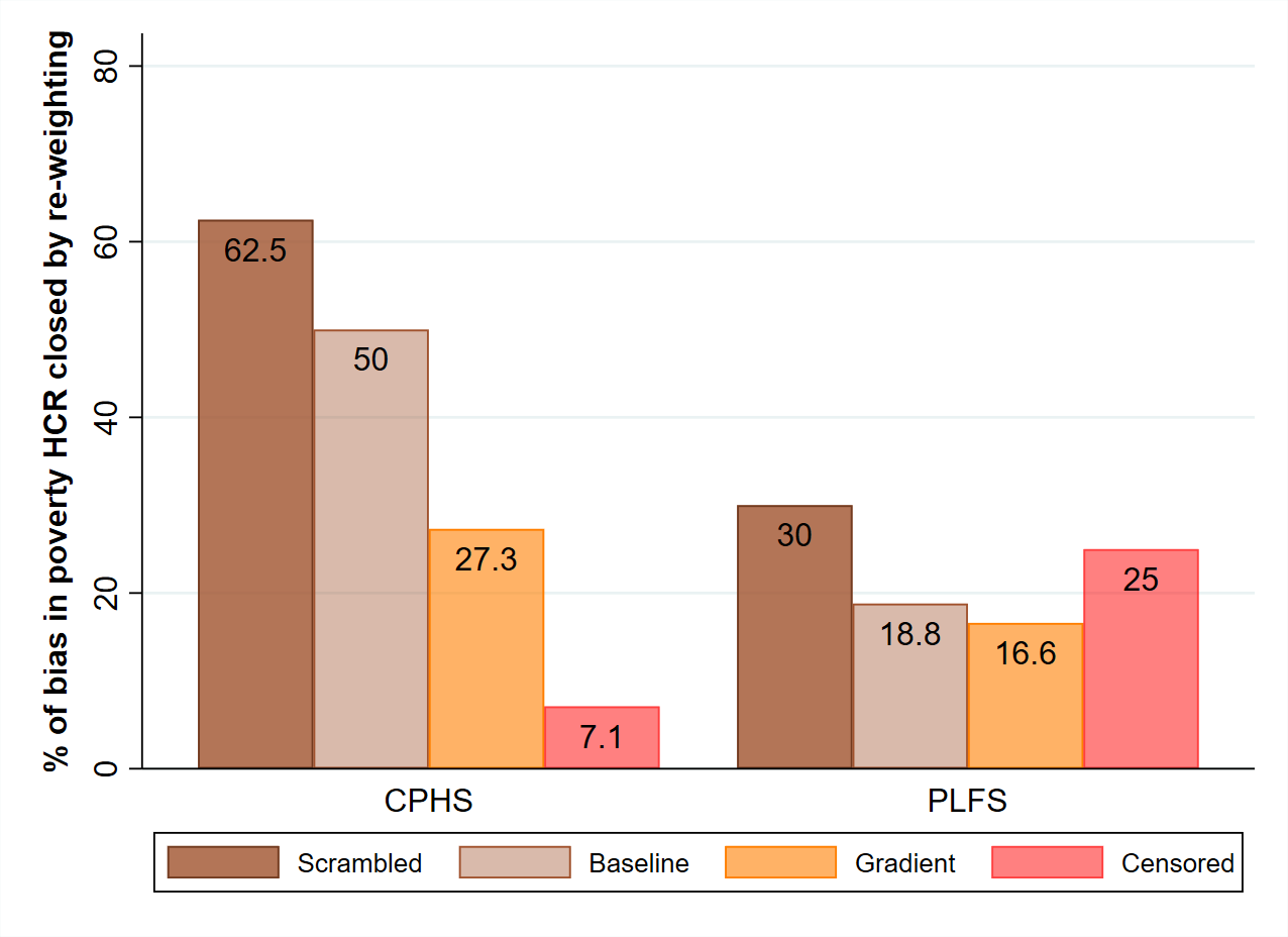
Note: The figure presents the proportion (in %) of gap between true and estimated poverty head-count ratio that max-entropy re-weighting closes on average in each of the contamination variants.
We tried many other variants of the simulations presented here, without learning much more. The basic point remains that the effectiveness of the max-entropy method (in terms of percentage reduction in the difference between true and estimated focus statistics) is uncertain and varies a great deal between contamination variants. One pattern of interest is that the effectiveness of the method declines as the proportion of poor households being dropped increases. If that proportion is higher than the true head-count ratio, so that the contaminated sample has no poor households at all, then the max-entropy method is virtually useless. As one colleague aptly put it, “you cannot re-weight yourself out of situations where there are no representatives of the group you are interested in”.
Estimating poverty trends
Before concluding, we note that RW’s main purpose was to estimate poverty trends beyond the 2011-12 CES round of the National Sample Survey (NSS). For this purpose, they attempted not only to correct biases in the CPHS sample (from 2015 onwards), but also to address the fact that CPHS expenditure data may not be comparable with NSS data for 2011-12.
They do this by imputing NSS-type consumer expenditure to CPHS households (instead of taking the CPHS expenditure figures at face value), based on two different approaches. In the first, NSS-type consumer expenditure is predicted using household characteristics for each CPHS household based on a model derived from NSS 2011-12 data.10 In the second, NSS-type expenditure is imputed directly from CPHS expenditure by imposing distributional assumptions and then using the method of moments. Both approaches add another layer of approximation to their estimation of poverty levels and trends. The results are interesting, but it is hard to guess how reliable they are. Their seeming precision – for example, in RW’s summary statement that “extreme poverty is 12.3 percentage points lower in 2019 than in 2011” – is certainly difficult to reconcile with these multiple layers of approximation.
We can actually say a little more. RW’s poverty estimates assume that the underrepresentation of poor households in CPHS data is fully corrected by the max-entropy method. In fact, our simulation exercises suggest that the correction is only partial, and possibly far from a full correction. If so, RW’s estimates are likely to understate poverty in 2015-19, and overstate poverty decline between 2011-12 and 2019.
There is another crucial problem with the estimation of poverty trends from CPHS data: the underrepresentation of poor households seems to have grown over time in recent years.11 Moreover, as noted earlier, repairing this gap tends to get harder as the gap gets larger – just like socks are harder to mend when the hole is wider. Thus, growing underrepresentation of poor households could easily create an illusion of poverty decline. Figure 2 presents one major hint of this. Quite likely, the precipitous decline of adult illiteracy between 2015 and 2019 (from 25% to 3% in just four years!) reflects the growing underrepresentation of underprivileged households in CPHS data.12 Further, there is a striking co-movement between the trends in adult illiteracy and RW’s adjusted poverty estimates. For all we know, the decline of adjusted poverty estimates in that period may well be an artefact of the growing bias in CPHS data.
Figure 2. Trends in adult illiteracy rate and adjusted headcount ratio

Notes: i) Poverty estimates are taken from Roy and van der Weide (2022), Figures 15 and 17. ii) Adult illiteracy rates are estimated from unit-level CPHS data using original design weights (scaled by a non-response factor) for each of the three waves of each year and then averaged across waves.
RW’s analysis ends in 2019, just before the Covid-19 crisis. What happened after that is unclear as things stand, but it almost certainly includes a sharp increase in poverty in 2020 (Azim Premji University 2021, World Bank 2022).
Concluding thoughts
A number of salutary lessons emerge from this exercise. First, it is possible for a sample to miss many poor households without this showing clearly in observable socioeconomic variables – including correlates of MPCE. This reinforces our earlier concerns about the credibility of CPHS data for poverty estimation: the observable biases may well be associated with a huge underrepresentation of poor households.
Second, the effectiveness of the max-entropy method depends critically on the nature of the biases it attempts to correct. It may work reasonably well when the bias takes the form of households missing at random from observable groups. However, it is hard to know in advance (or even in hindsight) whether that is the case.
Third, it is one thing to correct mean MPCE, and quite another to correct a distribution-sensitive MPCE statistic like the headcount ratio.13 RW’s implementation of the max-entropy method focuses on control means, but any aspect of the joint distribution of control and focus variables potentially matters.
Fourth, estimates of Indian poverty levels and trends based on the max-entropy method have an unknown and possibly wide margin of error. The method has been greeted with enthusiasm by the World Bank and others, but the proof of the pudding is still awaited.
Fifth, these estimates are likely to exaggerate the extent of poverty decline between 2011-12 and 2019. For one thing, the max-entropy method does not fully correct for the underrepresentation of poor households in CPHS data for 2015-19. For another, the underrepresentation of poor households was growing within that period, creating a spurious source of decline in poverty estimates. To paraphrase RW, poverty in India has probably declined over the last decade (up to the Covid-19 crisis), but how fast is anyone’s guess.
Sixth, the concerns raised here potentially apply to a range of contexts, beyond just poverty estimation. Re-weighting on observables is often used to correct for selection bias. The assumptions required for this method to produce good results are reasonably clear from the technical literature, but they are sometimes overlooked in practical applications.
Finally, major doubts remain about the credibility of the CPHS dataset as a nationally representative household survey. The nature of the CPHS biases, and the extent to which they can be corrected, are yet to be fully understood.
The silver lining is that another CES round is expected later this year. If it is released in good time without tinkering, it may shed some light on poverty trends and also facilitate closer scrutiny of the max-entropy method. In the meantime, we remain largely in the dark.
We are grateful to Angus Deaton, Parikshit Ghosh, Thiago Scarelli, Sutirtha Sinha Roy and Roy van der Weide for insightful comments on an earlier draft; Sutirtha Sinha Roy also contributed helpful clarifications on max-entropy re-weighting.
Notes:
- The NFHS figure for toilets actually refers to ‘access to any toilet’ (including shared facilities). This accentuates the contrast between the two sources.
- For earlier comments on this method and related issues, see Himanshu (2022), Ravallion (2022), Sandefur (2022), and other contributions to the recent Ideas for India e-Symposium on “Estimation of Poverty in India” (Ghatak 2022).
- When the original weights are uniform (that is, all households have the same weights), maximising entropy implies finding adjusted weights that are as uniform as possible, subject to meeting the specified control means. The extension used by RW, for unrestricted original weights, consists of “minimising cross-entropy”. See Golan (2006) and Wittenberg (2010) for further details.
- In a simple case where individuals possess just two binary characteristics, one observable and the other not, it can be shown that re-weighting produces a representative sample if and only if the two characteristics are perfectly correlated; if not, biases will remain (Somanchi, forthcoming).
- These sorts of concerns seem to be well acknowledged in the literature. To quote Brick and Kalton (1996) – “While these methods are generally beneficial, they are inevitably imperfect. They rely on assumptions, such as the MAR [missing at random] assumption, that are questionable and difficult to empirically verify. Thus these compensation methods should not be viewed as a substitute for obtaining valid responses.”
- Here, MPCE refers to ‘usual’ household consumption expenditure as recorded in PLFS. This is not strictly comparable with MPCE as defined in NSS or CPHS surveys, but that does not matter for our simulation exercise.
- We use only household-level variables as control variables and adjust weights at the household-level. All members of a household are assigned the same adjusted weight for the purpose of estimating the poverty head-count ratio.
- The mean of a dummy variable is the proportion of households for which the dummy takes value 1 – for example 9% for the ST dummy in the full sample (Table 1, first entry).
- A similar point is made by Andrews and Oster (2018) in the context of external validity of estimates from treatment effect models: “If participation is driven entirely by observable variables, this problem has a well-known solution; one can re-weight the sample to obtain population-appropriate estimates. However, when participation depends on unobservable factors, including directly on the treatment effect, adjusting for differences in observable characteristics may be insufficient.”
- The household characteristics used for imputation are demographics, education, employment, asset ownership and dummies for non-zero expenditure on four specific consumption categories.
- The gap between CPHS and other sources has widened considerably over the 2014-2019 period, with CPHS showing much faster rates of progress over time on various indicators; see Drèze and Somanchi (2021), and Tables 3a and 3b in Somanchi (2021) for further details.
- According to National Family Health Survey data (NFHS-3 and NFHS-4), adult illiteracy declined by about one percentage point per year between 2005-06 and 2015-16. We are not aware of any developments that would explain a dramatic acceleration after that, and there is no sign of acceleration in the latest NFHS round for 2019-20.
- This is all the more so when the headcount ratio is a little ‘volatile’ owing to many households being bunched just above or below the poverty line; see Deaton and Drèze (2002) on the “density effect”. It is also worth noting that adjusting mean MPCE could be particularly ineffective when there are missing households at both ends of the distribution (richest and poorest).
Further Reading
- Aguilar, R, et al. (2022), ‘September 2022 Update to the Poverty and Inequality Platform (PIP): What’s new’, World Bank Global Poverty Monitoring Technical Note 24.
- Andrews, I and E Oster (2018), ‘Weighting for External Validity’, NBER Working Paper 23826.
- Azim Premji University (2021), ‘State of Working India 2021: One year of Covid-19’, Centre for Sustainable Employment, Azim Premji University.
- Brick, JM and G Kalton (1996), “Handling missing data in survey research”, Statistical Methods in Medical Research, 5(3): 215-238.
- Deaton, Angus and Jean Drèze (2002), “Poverty and Inequality in India: A Re-examination”, Economic and Political Weekly, 37(36): 3729-3748. Available here.
- Deville, Jean-Claude and Carl-Erik Särndal (1992), “Calibration Estimators in Survey Sampling”, Journal of the American Statistical Association, 87(418): 376-382.
- Drèze, JP and A Somanchi (2021), ‘New Barometer of India’s Economy Fails to Reflect Deprivations of Poor Households’, Economic Times, 21 June.
- Ghatak, M (2022), ‘Introduction to e-Symposium: Estimation of Poverty in India’, Ideas for India, 10 October.
- Golan, Amos (2008), “Information and Entropy Econometrics – A Review and Synthesis”, Foundations and Trends® in Econometrics, 2(1-2): 1-145. Available here.
- Himamshu (2022), ‘Statistical Priorities for the ‘Great Indian Poverty Debate 2.0’, Ideas for India, 15 October.
- Ravallion, M (2022), ‘Filling a gaping hole in World Bank’s global poverty measures’, Ideas for India, 14 October.
- Roy, SS and R van der Weide (2022), ‘Poverty in India Has Declined Over the Last Decade But Not as Much as Previously Thought’, World Bank Policy Research Working Paper 9994.
- Sandefur, J (2022), ‘The Great Indian Poverty Debate, 2.0’, Ideas for India, 12 October.
- Somanchi, A (2021), ‘Missing the Poor, Big Time: A Critical Assessment of the Consumer Pyramids Households Survey’, SocArxiv.
- Somanchi, A (forthcoming), ‘Weighting the evidence: Poverty Estimation with Biased Samples’, SocArxiv.
- Wittenberg, Martin (2010), “An introduction to maximum entropy and minimum cross-entropy estimation using Stata”, The Stata Journal, 10(3): 315-330.
- World Bank (2022), ‘Poverty and Shared Prosperity 2022: Correcting Course’, World Bank.

By: Mohamad Aslam 16 July, 2024
In the second table, mean mpce- is it calculated by taking consumption data for all the items, for September, October, November and December together? Or for a specific month? As a researcher I am exploring these data sets and want to learn these methods. Is it possible to learn applied simulation in this paper, or software commands? Dr. Mohamad Aslam Postdoctoral Fellow, IISER, Mohali (India)