

 13 October, 2022


In the fourth post of a six-part series on the estimation of poverty in India, Sinha Roy and van der Weide reflect on the dramatically different estimates produced by two studies, and the source of the discrepancy. They put the estimates from the papers side by side in order to investigate three likely causes for this – using consistent data sources to determine pass-through rates, incompatibility in pass-through and growth rate series, and the incorporation of subsidies into the calculations of household expenditure.
Official estimates of poverty in India are derived from the National Sample Survey (NSS) household Consumption Expenditure Survey (CES). The most recent CES was compiled back in 2011, so to estimate how poverty in India has evolved since then, alternative sources of data (and accompanying prediction methods) are required. Earlier this year, two working papers came out, coincidentally within a day from each other, that produced estimates of poverty for India using different sources of data.
The first of these studies is a World Bank working paper by the authors of this blog (Sinha Roy and van der Weide, henceforward referred to as RW), which uses the new Consumer Pyramid Household Survey (CPHS) collected by the private sector to measure consumption poverty. The CPHS is the first household survey collecting detailed household expenditure data since the official CES round of 2011. Its expenditure questionnaire is, however, not readily comparable to that of the CES. For this reason, we estimate the relationship between CPHS and CES household consumption and use this to convert CPHS consumption data into NSS-compatible consumption data, such that estimates of poverty and inequality obtained using the CPHS for the period 2015-2019 can be compared against historical poverty and inequality estimates until 2011.
The second study is an IMF working paper by Bhalla, Bhasin and Virmani (henceforward referred to as BBV), which uses state-level GDP growth data to project mean household consumption growth. It works under the assumption that state inequality levels have remained unchanged over this time period (as state-level GDP data does not offer an any information on distributional changes).
Comparing poverty estimates
Figure 1 shows the poverty estimates from RW and BBV side by side, where the solid red line represents our reproduction of BBV following the approach outlined in their paper. The two studies are seen to paint a markedly different picture of how headcount poverty, the population share whose consumption lies below the World Bank’s poverty line of $1.90 a day (in 2011 purchasing power parity (PPP)), has evolved over the last decade.
Figure 1. Replicating the BBV headcount estimates
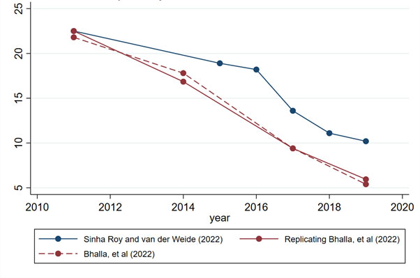
Notes: i) Our replication of BBV starts with the empirical nominal consumption distribution denominated in Uniform Recall Period (URP) terms from the 2011 CES. ii) Mean household consumption at the state level for the years following 2012 is estimated using growth rates in per capita gross state domestic product, assuming distribution neutrality within the state, and unity pass-through. iii) State-level population estimates are based on projections from national accounts.
While both studies estimate a decline in poverty, they disagree on the magnitude of extreme poverty in India. BBV estimate that in 2019 about 5% of India’s population lived in extreme poverty. This is half the extreme poverty rate estimated by us. This apparent divergence between the poverty estimates is reminiscent of the ‘Great Indian Poverty Debate’ from the 1990s (see for example, Deaton and Kozel 2005), prompting Justin Sandefur (2022) to refer to today’s debate as the ‘Great Indian Poverty Debate, 2.0’.
It should be expected that different data and methods will yield different results. Yet, the magnitude of the difference in estimated poverty rates demands a reflection on the sources of the discrepancy.
Investigating pass-through rates
A possible explanation stems from the fact that poverty projections are highly sensitive to the value of the pass-through rate that governs the relationship between mean household consumption growth and GDP growth. Different choices of GDP growth series will generally have different pass-through rates (that is, they will have a different relationship with mean household consumption growth). BBV find that household consumption and national consumption from national accounts (NA) were growing at approximately the same rate between 2004 and 2011. Based on this empirical observation, BBV estimate the pass-through rate to be 1, which is somewhat higher than estimates documented in the existing literature based on cross-country regressions. Rather than assuming that national GDP growth and state GDP per capita growth share the same pass-through rate (as BBV do), one would ideally work with an estimate for the series that is used to project mean household consumption growth levels (which, in the case of BBV, is the growth in nominal gross state domestic product (GSDP)).
Given the significance of the pass-through rate for the approach adopted by BBV to estimating poverty, let us estimate it by regressing mean household consumption growth on state GDP growth for the 2004-2011 period. This yields an estimate of 0.916 for the pass-through. While this is very close to the unit pass-through assumed by BBV, and within the range of historical pass-through estimates they identified, this modest difference is shown to make a meaningful difference for estimates of poverty. Our data also allows us to account for heterogeneity in pass-through by computing separate pass-through rate for each state (simply by dividing mean household consumption growth by state GDP growth for each state). The resulting poverty trends for both choices are shown in Figure 2, where the only change we have made is adjusting the value of the pass-through rate (all else is kept the same as in BBV).
Figure 2: Estimates of poverty headcount (at $1.90 PPP) based on state GDP specific pass-through rates
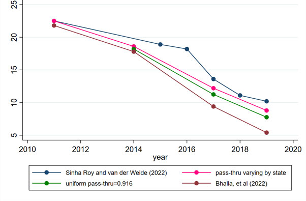
Notes: i) Uniform pass-through of 0.916 is estimated by regressing growth in state-level nominal consumption per capita, using the 2011 and 2004 rounds of CES, on growth in nominal state GDP per capita over the same period. ii) The state-specific pass-throughs are estimated by the ratio of nominal survey consumption per capita growth and the nominal state GDP per capita for 2004 and 2011.
It follows that the divergence in poverty rates between RW and BBV can largely be accounted for by adopting estimates of the pass-through rate fitted to the state GDP series. Using the uniform (or average) pass-through of 0.916 (from the cross-state regression) approximately halves the gap in poverty rates between RW and BBV. Accounting for between-state differences in pass-through comes close to eliminating the gap completely. One difference between the two estimated poverty trends that continues to stand out is the break in the trend around 2016 – corresponding to demonetisation in India – which can be observed in our estimates, but not in the estimates by BBV.
Incorporating food subsidies into the poverty calculation
Another innovation adopted by BBV is that they value household expenditures on subsidised rice and wheat at market prices (rather than at the subsidised prices households purchased the rice and wheat for). This is by no means an unreasonable choice. It should be noted however, that this approach implies abstracting from quality differences between goods. To illustrate this, we regress the unit price of four choices of goods (rice, wheat, milk, and salt) against log household expenditure from the 2011 CES of the NSS (see Figure 3). All expenditures concern market goods (that is, the purchase of subsidised rice and wheat are excluded). The slopes of the fitted lines arguably capture differences in both quality and location. Salt is included as a control as it represents the most homogenous good among the four, with little to no variation in quality, such that the slope coefficient captures variation in location, not quality. Subtracting this slope for salt from the slopes observed for rice, wheat, and milk indicates that a notable degree of the variation in prices can be attributed to quality differences – richer households on average purchase higher quality versions of the same good at higher prices.1
Figure 3. Differences in unit prices for the same item, in rural (left panel) and urban households (right panel)
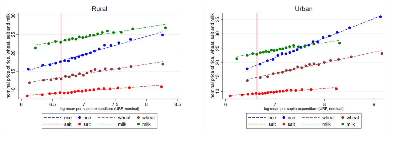
Notes: i) The upward slopes here capture the higher nominal prices paid by households for the same good at different per capita expenditures. These are arguably induced by differences in the quality of staples purchased at different expenditure levels when compared to the slope of salt. ii) Unit prices are calculated as the ratio of household expenditure on items and quantities consumed in the 2011 round of CES. iii) The unit price for rice and wheat depicted in the figure does not include households’ cereal consumption from the Public Distribution System (PDS). iv) The vertical red line is the $1.90 poverty line – poor households are to the left of this line
Implications
Abstracting from quality differences for the purpose of poverty measurement is certainly a defensible choice. However, this choice has several important implications that warrant further study.
First, virtually every consumption good can be purchased at different quality levels, and consequently exhibit variation in unit prices. Hence a consistent application of this approach would require one to apply the price adjustments across a wider set of goods (not just subsidised rice and wheat).
Second, what price should one value the expenditures at for the poverty estimates? The average market price assumed by BBV is generally significantly higher than the average price households below or around the poverty line purchase the goods for in rural areas (see Figure 4). In urban areas, the assumed uniform prices are notably closer to (or just below) the nominal unit price paid by poor households.
The figure shows that in rural areas, the implied unit price of rice based on observed prices in 2011 NSS and state level CPI food indices (the preferred deflator series in BBV) is lower than the price rice assumed by BBV across the years following 2011. This discrepancy will overestimate poverty reduction in rural areas but underestimate poverty reduction in urban. Since discrepancies are markedly larger in rural samples and rural population is about 67% of the overall population, the national poverty estimates at BBV’s assumed price levels likely overestimate average consumption and underestimate national poverty headcounts.
Figure 4. Impact of selection of a uniform market price on poverty estimates
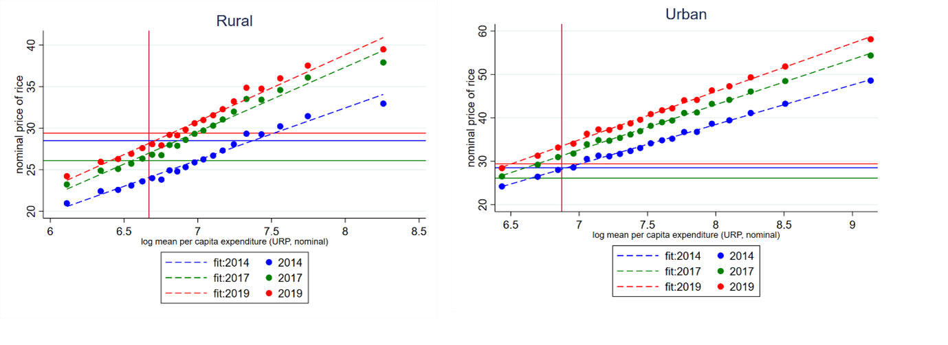
Notes: i) Unit prices for 2014, 2017 and 2019 are calculated using the observed unit price of rice in the 2011 CES, and the food price inflation reported in the CPI state (rural and urban) series – BBV’s preferred choice of deflator series. ii) The horizontal lines in different colours represent the price at which BBV value PDS consumption of rice. iii) The vertical red line is the $1.90 poverty line – poor households are to the left of this line.
Third, the same price that is used to adjust household expenditure values should ideally also be used to adjust the value of the national poverty line. For example, the amount of rice included in the basic needs basket that underlies the poverty line should be evaluated at the same price. Using subsidised prices to value the poverty line but higher market prices to value household expenditures (as BBV currently do) will lead to an under-estimation of poverty. It should be noted that BBV adopt the international poverty line of $1.90 a day, and hence do not have to evaluate the price of the basic needs consumption basket for India. By the same token, however, the international poverty line is derived from cross-country data on poverty lines that reflect the cost of acquiring the basic needs basket. Conceptually, this means that if one were to change the prices used to evaluate household expenditures, one would have to use the same prices to evaluate the cost of the basic needs basket to verify whether households can afford the basic needs consumption basket.
Additional comments: BBV suggest that the targeting efficiency of India’s PDS program improved from 54% to 86% from 2014-15 onwards, citing data on the coverage of food transfers during the pandemic from Bhattacharya and Sinha Roy (2021) in support of their projections. As a point of clarification, Bhattacharya and Sinha Roy (2021) finds that a high share of people across the welfare distribution were able to receive government transfers (while taking stock of the PDS transfers during the emergency covid period). For instance, 93.1% of poor eligible households received these transfer benefits in addition to 81% of eligible non-poor households. From these estimates alone, one cannot infer with what efficiency PDS transfers are allocated across households with different expenditures – and hence are not able to provide support for the assumed targeting efficiency estimate of 86% in BBV.
The authors are grateful to Andrew Dabalen, Christoph Lakner, Daniel Mahler, Berk Ozler, Carolina Sanchez Paramo for providing helpful comments and suggestions.
A version of this article previously appeared on the Center for Global Development (CGDev) blog.
Notes:
- Deaton (1988) puts forward an approach to account for these quality differences.
Further Reading
- Bhalla S, K Bhasin and A Virmani (2022), ‘Pandemic, Poverty, and Inequality: Evidence from India’, International Monetary Fund, IMF Working Paper No. 2022/069.
- Deaton, Angus (1998), “Quality, Quantity, and Spatial Variation of Price”, The American Economic Review, 78(3): 418-430.
- Deaton, Angus and Valerie Kozel (2005), “Data and Dogma: The Great Indian Poverty Debate”, The World Bank Research Observer, 20 (2): 177-200.
- Sandefur, J (2022), ‘The Great Indian Poverty Debate, 2.0’, Ideas for India, 12 October.
- Roy, SS and R van der Weide (2022), ‘Poverty in India Has Declined over the Last Decade But Not As Much As Previously Thought’, World Bank, Policy Research Working Paper No. 9994.

Comments will be held for moderation. Your contact information will not be made public.