The combined stock of debt owed by Indian states is about 21% of GDP, and is proliferating. In this article, Ananya Kotia discusses why the stock of the states’ debt is unsustainable today despite their commendable adherence to hard limits on borrowing flows imposed by India’s fiscal rule framework.

The combined stock of debt owed by the Indian states is about 21% of GDP (gross domestic product) (excluding UDAY (Ujwal DISCOM Assurance Yojana) bonds) today, and is proliferating unsustainably. Higher borrowing (fiscal deficit) by the states, even though it remains within the annual target of 3% of GDP, threatens the sustainability of subnational debt at present levels.

India’s fiscal rule framework imposes legal limits of 3% of GDP on the fiscal deficits of the central and all state governments. Adhering to these borrowing limits, though prudent economics, makes for difficult politics as expenditure is curtailed. It is therefore a significant achievement that Indian states have largely operated within their 3% fiscal deficit limits in the past decade.

This raises a paradox: why is the states’ debt unsustainable today despite their commendable adherence to hard borrowing limits? Though high primary deficit of the states is one reason, there is also a deeper, conceptual reason for the states’ deteriorating debt levels.

Internally inconsistent fiscal rules

The fault lies not in the inadequate implementation of fiscal rules by the states but in the design of these rules themselves. A 3% cap on fiscal deficit is too high to stabilise the states’ debt around the desired level of 20%. Why then was the states’ fiscal deficit target set at this level?

Though an insubstantial, post-facto justification, based on simplistic fiscal arithmetic, came from the 12^th Finance Commission, the level of the states’ fiscal deficit target was probably kept at 3% to make it politically palatable by maintain equality with the Centre’s deficit target.

But the symmetry in the deficit targets for the states and the Centre was, and remains, inconsistent with the widely divergent debt levels of the two tiers of the government. While the annual fiscal deficit targets of 3% of GDP are equal for both the centre and the states, experts within the government and outside, have argued for an unequal division of general government (states plus the central government) debt: with 40% apportioned to the Centre and the residual 20% to the states. Thus, by design, India’s fiscal framework creates a tension between the equal targets for annual flows of borrowing (that is, fiscal deficit) on one hand and the unequal levels of the desired stock of accumulated borrowing (that is, debt) on the other.

The importance of the level of debt

What matters for macroeconomic stability is not the value of debt in rupees but the magnitude of debt relative to the magnitude of GDP, that is, the debt-GDP ratio. In a country with high nominal GDP growth, like India, this has key implications on how fiscal data are interpreted. As GDP grows rapidly, it partially erodes the debt-GDP ratio each year because even if debt rises in magnitude (due to fresh borrowing), it shrinks in proportion to GDP.

Consider the standard equation of the law of motion of the debt-GDP ratio:

d_t=1/(1+γ) d_(t-1)+f_t

where d_t is the debt-GDP ratio in period t; γ is the nominal growth rate of GDP; f_t is the fiscal deficit to GDP ratio in period t.

The equation says that the debt-GDP ratio in period t is the sum of the debt-GDP ratio in period t-1 that is not eroded by nominal GDP growth plus the fiscal deficit-GDP ratio in period t. γ/(1+γ) is the rate at which past debt is eroded due to nominal GDP growth such that (1-γ/(1+γ)) or 1/(1+γ) of past debt carries on to the next period. If we measure both central government and subnational debt relative to GDP, this rate of erosion is the same for the two tiers of government. However, the base, that is, the debt-GDP ratio, to which this rate is applied, is much larger for the Centre. This difference in the initial levels of debt between the two tiers of the government has self-evident implications for the design of their fiscal rules.

For example, at present levels of nominal GDP growth of 11-12%, about 11% of the debt-GDP ratio is eroded each year merely on account GDP growth. In the previous fiscal year (FY17), this was over 5 percentage points of the central government’s debt ratio of 49.4% of GDP. Therefore, despite fresh borrowing of 3.5% of GDP last year, which added to the magnitude of debt, the centre’s debt-GDP ratio decreased from 49.4% in FY17 to 47.4% of GDP in FY18. How? Because between FY17 and FY18, GDP growth eroded as much as 5.5 percentage points from the central government’s debt-GDP ratio.

The states however, are not so lucky. GDP growth erodes their debt-GDP ratio by only 2.1 percentage points, less than half as compared to the Centre. Like in the case of the central government, this is about 11% of their present debt-GDP ratio of just over 20% of GDP. The rate of erosion (that is, 11%) is the same for both tiers of the government. However, in the case of the states, this erosion rate works on a much lower debt-GDP ratio of 20% of GDP, yielding a smaller annual growth-erosion as compared to that of the central government.

Implication for setting fiscal targets

Though counterintuitive, it follows therefore that the Centre can afford larger deficits because of its larger stock of debt alone. Symmetry cannot be forced on the targets for fiscal deficits of central and subnational borrowing given the significant difference in their present and desired stocks of debt. Any such attempt will simultaneously induce the debt-GDP ratios of the two tiers of government to converge. Currently, at around 3% of GDP, the states are borrowing more than their annual erosion of debt due to nominal GDP growth. If this trend continues, their debt-GDP ratio will continue to rise, eventually stabilising at around 30% − far above the desired level.

Figure 1. Debt projections under present fiscal responsibility legislation (FRL) and alternative scenario for the Centre and the states

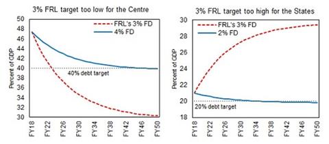
If both the centre and the states were to operate at their fiscal responsibility legislation (FRL) limits of 3% (as is the situation today), both the central and the subnational debt-GDP ratios will stabilise at 30%. For the states, this implies a sharp, sizeable jump in their debt, even if they adhere to their FRL deficit limits. If the desired level of state debt is about 20%, then the states should be subjected to a lower deficit ceiling. A deficit ceiling of 2% (blue line in Figure 1) will suffice to stabilise the states’ debt at this level. On the other hand, if the central deficit remains at 3%, its debt ratio will continue to decline until it stabilises at 30% − far lower than desired.

The 15^th Finance Commission − which is likely to be set up soon − must amend fiscal rules to maintain consistency between stock and flow variables.

An earlier version of this article appeared in the Business Standard on 7 July 2017.

Note:

1. I assume nominal GDP growth of 11.11% (equal to the CAGR (compounded annual growth rate) of the past five years, that is, from 2012-13 (99,440 bn) to 2016-17 budget estimates (168,475 bn). The projections are based only on equation (1) above. The starting values (FY18) of the debt-GDP ratios are 47.4% for the Centre and 21% for the states.