In Part I of this two-part series, the authors presented their estimates of total budget subsidies, and their merit and non-merit components. In this part, they discuss the relationship between subsidies and the delivery of specific public services, the comparative efficiency of subsidy use by different states, and the scope for rationalisation of subsidies as a part of deep fiscal reforms, in order to create fiscal space for reviving inclusive growth following the Covid-19 lockdown shock.

Subsidies and service delivery

In an earlier paper, Mundle et al. (2016) had developed indicators of public service delivery in major Indian states. These and other indicators have been combined with the estimate of per-capita subsidies for specific public services to assess the relationship between subsidies and public service delivery. It turns out that there is a significant positive relationship between subsidies and delivery of many – but not all – public services. Some examples follow.

Among infrastructure services, there is a strong positive relationship between per-capita transport subsidy and state highway density (kms per 100 square km), which is statistically significant at 1% level (Figure 1). However, the relationship between power subsidy and per-capita consumption of electricity (kilowatt hour (kWh)) is not statistically significant.

Figure 1. State highway density and per-capita transport subsidy, 2011-12

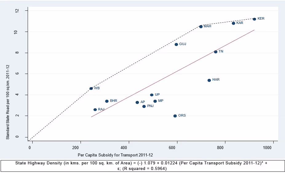
Notes:

(i) * Significant at 1% level;

(ii) State codes: AP-Andhra Pradesh (Telangana); BHR-Bihar (includes Jharkhand); GUJ-Gujarat; HAR-Haryana; KAR-Karnataka; KER-Kerala; MP-Madhya Pradesh (includes Chhattisgarh); MAH-Maharashtra; ORS-Orissa; PNJ-Punjab; RAJ-Rajasthan; TN-Tamil Nadu; UP-Uttar Pradesh (includes Uttarakhand); WB-West Bengal

(iii) State highway density is measured in terms of kms per 100 sq. km of area.

Among social services, there is a strong positive relationship between education subsidies and different indicators of educational outcomes. The relationship between per-capita education subsidy and literacy rate (2011-12), and the government’s education development index (Education Development Index, 2011-12)¹ are presented in Figures 2a and 2b, respectively. The relationship of per-capita education subsidy with both indicators is positive and statistically significant at the 1% level. A similar strong positive relationship is evident between education subsidy and learning indicators for reading and mathematics, both again significant at the 1% level, as can be seen in Figure 3a and 3b². The indicators selected are measures of the reading and mathematics skills of students of grade 1 and 2.

Figure 2a. Education service delivery (literacy rate) and per-capita education subsidy, 2011-12

Notes:

(i)* Significant at 1% level.

(ii) State codes: same as Figure 1.

Figure 2b. Education service delivery (Education Development Index (EDI)) and per-capita education subsidy, 2011-12

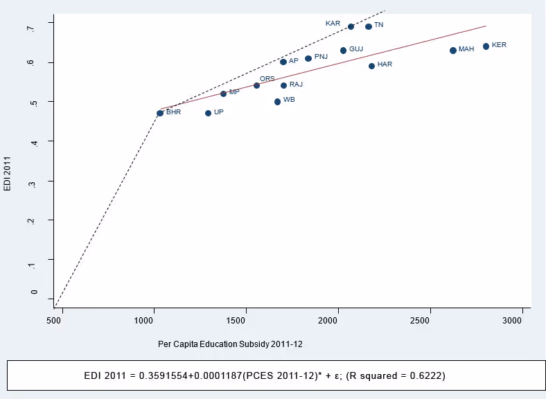
Notes:

(i) * Significant at 1% level;

(ii) State codes: same as Figure 1.

Figure 3a. Education service delivery (ASER reading level for grade 1-2 in 2011) and per-capita education subsidy, 2011-12

Notes:

(i) * Significant at 1% level.

(ii) State codes: same as Figure 1.

Figure 3b. Education service delivery (ASER math level for grades 1-2 in 2011) and per-capita education subsidy, 2011-12

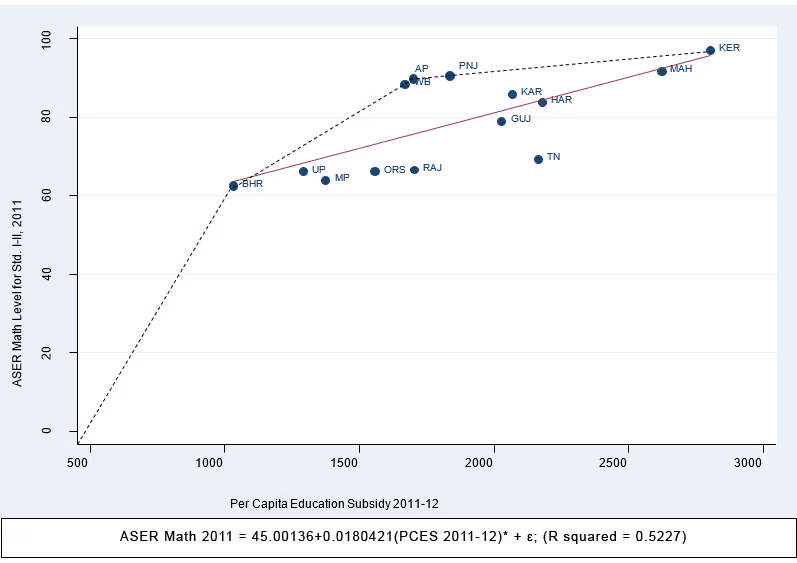
Notes:

(i)* Significant at 1% level.

(ii) State codes: same as Figure 1.

The relationships between per-capita subsidy for consumption of health services and health outcome indicators, namely, the Infant Mortality Rate (IMR) and life expectancy are presented in Figures 4a and 4b respectively. The two indicators have an inverse and a positive correlation with per capita healthcare subsidy, both again significant at 1% level.

Figure 4a. Health service delivery (infant mortality rate) and per-capita health subsidy, 2011-12

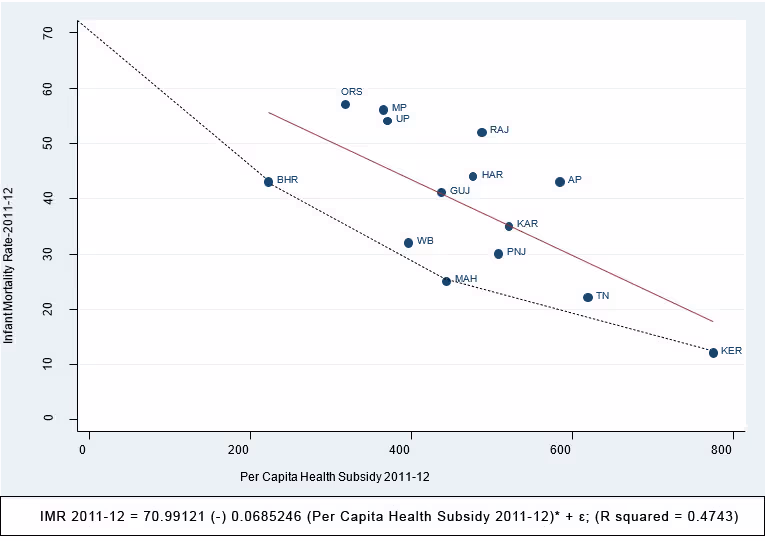
Notes:

(i)* Significant at 1% level.

(ii) State codes: same as Figure 1.

Figure 4b. Health service delivery (life expectancy at birth, 2009-13) and per-capita health subsidy, 2011-12

Notes:

(i)* Significant at 1% level.

(ii) State codes: same as Figure 1.

The key policy takeaway from this evidence is that key public services, such as education, health, and road infrastructure are significantly correlated with the service-specific per-capita subsidy. However, correlation is not causality and that could run either way. Subsidy could be driving higher consumption of the service or higher consumption of a service at less than full-cost recovery may lead to higher subsidies. Either way, it implies that public action to enhance the consumption of these services – especially merit services – will require a higher volume of subsidies.

Inter-state variation in subsidy efficiency

Another issue related to service-specific subsidies is the efficiency of these services. We find that here are large variations in the efficiency of service-specific subsidy use across states. The hatched lines in Figures 1, 2a and 2b, 3a and 3b, 4a and 4b trace the convex curves (concave in 4a), which define the boundaries of the ‘revealed efficiency frontier’ for various service-specific subsidies. States at the vertices of these curves are states that lie on the subsidy efficiency frontier³. States that lie below the frontier (above in 4a) are inefficient. The vertical distance from the frontier is a measure of their inefficiency. To illustrate, for road density, the transport service indicator, West Bengal, Maharashtra, and Kerala lie on the frontier (the dashed line in Figure 1), while Gujarat and Karnataka are close to it. Others lie well below the efficiency frontier and Odisha is the furthest away from it, that is, it is the most inefficient.

States on the subsidy efficiency frontier include both low- and high-income states as well as low- and high-subsidy incidence states. The point to note is the large inter-state variation in efficiency levels. Since these are all states within the same country, with broadly similar levels of State capacity, it implies that there is much room for the less efficient states to improve their efficiency levels in delivery of various services by following the best practices of the more efficient states.

Non-merit subsidies and fiscal space

The Covid-19 pandemic and the subsequent stringent nationwide lockdown has delivered a very severe negative shock to an economy that was already decelerating quite sharply since 2018-19. In this context, we have often argued – as have many others – that in addition to ramping up health services on an emergency basis, the government also needs to substantially increase food and income support (Mundle 2019, 2020; Mundle and Sikdar 2019, 2020)⁴. The implied massive increase in expenditure would have a strong multiplier effect, which would help revive inclusive growth. However, to finance such additional expenditure when revenues have declined sharply, it is necessary to implement deep fiscal reforms that could free up the large fiscal space that is potentially available. These fiscal reforms should have three main components: to deal with non-merit subsidies, tax expenditures, and savings from excess appropriations.

Firstly, non-merit subsidies amount to over 5.7% of GDP (gross domestic product) (Table 1). Elimination of these unwarranted subsidies could free up considerable additional fiscal space. However, the bulk of these non-merit subsidies – over 4.1% of GDP – are actually being provided by the states. Hence, the rationalisation of these subsidies would mainly have to be undertaken by them. Second, a large volume of revenue is routinely foregone in the form of tax exemptions and concessions for both direct and indirect taxes. For the central government, this amounts to around 5% of GDP⁵. Third, there is a large volume of appropriated but unspent expenditure, amounting to around 1.5% of GDP for the central government (Comptroller and Auditor General (CAG), 2019). Thus, there is enormous potential but untapped fiscal space to finance a growth-reviving spending programme amounting to 12.2% of GDP. This is a lower-bound estimate since it excludes tax expenditure and excess appropriations of the state governments.

It would be unrealistic to assume that the entire potential fiscal space could actually be tapped. Perhaps it may not even be desirable in case of some tax concessions that induce extra savings, investment, etc. But if the government can commit itself to bold fiscal reforms to free up even half of the potential extra fiscal space, that would amount to a massive 6% of GDP. How should this extra fiscal space be used, especially to quickly put more money in the hands of poor consumers with a high marginal propensity to consume, to revive a process of inclusive yet fiscally prudent sustainable growth?

The expenditure package for such an inclusive growth revival strategy should have three main components:

(i) An income support programme: Ghatak and Muralidharan (2019) have made a compelling case for extending the PM-KISAN⁶ programme to all citizens without any targeting. They have estimated that such an expansion at the rate of Rs. 6,000 per household per year, would cost about 1% of GDP. We propose raising that to Rs. 200 per head per month, or Rs. 12,000 per year for a household of five persons at 2020-21 prices. This would amount to 2% of GDP. This should be additional to any existing income support programmes for specific target groups such as MNREGA⁷ (Mahatma Gandhi National Rural Employment Guarantee Act), scholarships, old-age pensions, etc. – and not a substitute for them. If it is considered unpalatable or politically inappropriate to make such universal support available for the rich, however insignificant it may be fiscally, it would be best to have a transparent negative list, for example, exclude all income taxpayers. This would be preferable to a positive target list that can be easily manipulated, with all its challenges of identification, leakage, and so on.

(ii) Additional expenditure on provision of health and education services, each amounting to 1% of GDP: The additional health expenditure should be used for ramping up the number of hospital beds, intensive care equipment and drugs, and for greater use of low-skilled health workers as force multipliers for doctors and nurses. The additional education expenditure should be used to scale up the quality of basic education, the most inclusive component of the recently announced National Education Policy.

(iii) Investment in infrastructure: The infrastructure deficit remains a major growth bottleneck in India. An extra allocation of 1% of GDP could be set aside for stepping up investment in road infrastructure, especially the Pradhan Mantri Gram Sadak Yojana (PMGSY) rural roads programme, which has been one of India’s most successful, employment intensive, infrastructure programmes.

The above three expenditure components would together use up extra fiscal space amounting to 5% of GDP. The balance of over 1% of GDP could be used to partly offset the recent decline in revenues. Thus, the expenditure and financing components of the deep fiscal reform programme outlined above would help to quickly revive inclusive growth without adding to the deficit. In fact, it would partly help offset the deficit impact of the sharp decline in revenues and without any increase in tax rates.

Table 1. Distribution of merit, non-merit, and total subsidies in social and economic sectors (% of GSDP/GDP)

	Merit subsidies						Non-merit subsidies						Total subsidies
State	Social sector			Economic sector			Social sector			Economic sector			Social sector			Economic sector			Total
	87-88	12-Nov	15-16	87-88	12-Nov	15-16	87-88	12-Nov	15-16	87-88	12-Nov	15-16	87-88	12-Nov	15-16	87-88	12-Nov	15-16	87-88	12-Nov	15-16
(0)	(1)	(2)	(3)	(4)	(5)	(6)	(7)	(8)	(9)	(10)	(11)	(12)	(13)	(14)	(15)	(16)	(17)	(18)	(19)	(20)	(21)
Andhra Pradesh (Telangana)	3.8	2.8	3.3	0.1	0.1	0.1	2	1.2	1.5	4	4.5	4.7	5.8	4	4.8	4.1	4.6	4.7	10	8.6	9.6
Bihar (includes Jharkhand)	6	4.2	4.4	0.3	0.1	0.2	1.8	1.4	1.5	7.2	5.7	5	7.8	5.6	6	7.5	5.8	5.3	15.3	11.4	11.2
Gujarat	4.1	3.3	3.2	0.1	0.1	0.1	1	0.9	0.7	4.6	2.5	3.1	5.1	4.2	3.9	4.7	2.6	3.2	9.7	6.8	7.1
Haryana	3.1	2.5	2.8	0.1	0.1	0.1	0.9	0.8	0.8	4.4	2.3	2.9	4	3.4	3.6	4.4	2.5	3	8.4	5.8	6.5
Karnataka	4	2.7	2.8	0.1	0.2	0.4	1.6	1.3	1.5	4.1	4.2	3.9	5.6	3.9	4.3	4.2	4.4	4.2	9.8	8.4	8.5
Kerala	4.7	2.9	2.8	0.2	0.3	0.3	1.3	1	1.7	2.7	1.8	1.7	6	3.9	4.5	2.9	2.1	2	8.8	6	6.5
Madhya Pradesh (includes Chhattisgarh)	4.9	4.1	4.8	0.2	0.2	1	1.7	1.1	1.9	4.6	4.4	4.1	6.5	5.2	6.7	4.8	4.6	5.1	11.3	9.8	11.8
Maharashtra	3.5	3	2.7	0.2	0.1	0.1	0.7	0.9	0.8	2.1	2.9	2.9	4.2	3.8	3.5	2.3	3	3	6.5	6.8	6.5
Orissa	3.8	3.4	4.5	0.2	0.5	0.5	1.5	1.3	1.1	4.7	3.6	3.7	5.3	4.7	5.7	4.8	4	4.2	10.1	8.7	9.8
Punjab	3.2	2.7	2.7	0.1	0	0.1	0.8	0.5	0.6	4.7	2.4	1.9	4	3.1	3.3	4.8	2.4	2	8.8	5.6	5.3
Rajasthan	4.9	4.8	5.1	0	0	0	0.9	0.6	0.8	6.2	2.2	3.1	5.8	5.4	6	6.2	2.3	3.1	12	7.7	9.1
Tamil Nadu	3.4	2.7	2.7	0.3	0.1	0.1	0.8	0.6	0.6	4.2	2.2	1.7	4.2	3.3	3.3	4.5	2.3	1.8	8.8	5.6	5.1
Uttar Pradesh (includes Uttarakhand)	3.4	4.4	4.3	0.2	0.3	0.2	0.9	0.8	1.7	4.3	4.5	5.5	4.4	5.2	6	4.4	4.8	5.7	8.8	10	11.7
West Bengal***	3.5	3.9	2.5	0.2	0.1	0.1	0.9	0.7	1	2.7	1.9	2.2	4.4	4.6	3.5	2.9	2	2.2	7.3	6.6	5.7
All states*	3.4	3	3	0.1	0.1	0.2	1	0.8	1	3.5	2.9	3.1	4.4	3.8	4.1	3.7	3.1	3.3	8.1	6.9	7.3
Centre*	0.3	0.9	0.2	0.7	1.5	1.1	0.3	0.1	0.2	3.5	1.3	1.4	0.7	0.9	0.4	4.2	2.8	2.5	4.9	3.8	2.9
All states + Centre*	3.7	3.9	3.2	0.9	1.6	1.3	1.3	0.9	1.2	7	4.3	4.5	5	4.8	4.5	7.9	5.9	5.8	12.9	10.7	10.3
All states' average**	4	3.4	3.5	0.2	0.2	0.2	1.2	0.9	1.2	4.3	3.2	3.3	5.2	4.3	4.6	4.5	3.4	3.5	9.7	7.7	8.2

Notes: (i) GSDP for 2011-12 and 2015-16 are at current prices in 2011-12 National Accounts Statistics (NAS) Series, whereas GSDP for 1987-88 are at current prices in 2004-05 NAS Series.

(ii) *These numbers are expressed in percentage of GDP.

(iii) ** All states’ averages are expressed in percentage of GSDP.

(iv) ***West Bengal’s GSDP for 2015-16 are collected from State Budget Speech, and 2011-12 GSDP is at current prices in 2004-05 NAS Series.

Notes:

1. Education Development Index (EDI), 2011-12 is a composite educational development index for all schools and managements, based on District Information System for Education (DISE) data, collected from NUEPA (2013), page 43.
2. The learning indicators are from various rounds of the Annual Survey of Education (Rural) Report (ASER).
3. The concept of a subsidy efficiency frontier is an adaptation of the states’ expenditure efficiency measure developed by Mohanty and Bhanumurthy (2018).
4. Food support through extra free rations has, in fact, been stepped up very significantly, though many citizens without ration cards have not been able to access the free rations. By comparison, steps to provide income support have been very limited so far.
5. See Annexure 7 of the 2020-21 central government receipts budget (Government of India, 2020).
6. PM-KISAN is a central-sector scheme that provides an income support of Rs. 6,000 per year to all farmer families across the country in three equal installments of Rs. 2,000 each after every four months.
7. MNREGA guarantees 100 days of wage-employment in a year to a rural household whose adult members are willing to do unskilled manual work at state-level statutory minimum wages.

Further Reading

• Comptroller and Auditor General of India (2019), ‘Accounts of the Union Government – Financial Audit, Report No. 2 of 2019’, 22 January 2019.
• Ghatak, M and K Muralidharan (2019), ‘An Inclusive Growth Dividend: Reframing the Role of Income Transfers in India’s Anti-poverty Strategy’, India Policy Forum, National Council of Applied Economic Research, 9 July.
• Government of India (2020), ‘Receipts Budget 2020-21’, Ministry of Finance, Budget Division.
• Mohanty, RK and NR Bhanumurthy (2018), ‘Assessing Public Expenditure Efficiency at Indian States’, National Institute of Public Finance and Policy (NIPFP) Working Paper No. 225, New Delhi, 19 March.
• Mundle, S (2019), ‘An Inclusive Strategy for India to Revive Its Economic Growth’, HT Mint, 17 October 2019.
• Mundle, S (2020), ‘Triple Trouble - Coronoavirus, hunger and the economy’, HT Mint, 17 April 2020.
• Mundle, Sudipto and Satadru Sikdar (2020), “Subsidies, Merit Goods and the Fiscal Space for Reviving Growth: An Aspect of Public Expenditure in India”, Economic & Political Weekly, 55(5):52-60, 1 February.
• Mundle, Sudipto and Satadru Sikdar (2019), “Inclusive Fiscal Adjustment for Reviving Growth: Assessing the 2019-20 Budget”, Economic & Political Weekly, 54(38):32-36, 21 September 2019.
• Mundle, Sudipto, Samik Chowdhury and Satadru Sikdar (2016), “Governance Performance of Indian States: Changes between 2001-02 and 2011-12”, Economic and Political Weekly, 51(36):55-64, 3 September 2016.
• Mundle, Sudipto and M Govinda Rao (1991), “Volume and Composition of Government Subsidies in India, 1987-88”, Economic & Political Weekly, 26(18):1157-1172, 4 May 1991.
• National University of Educational Planning and Administration (2013), ‘Elementary Education in India: Progress towards UEE, Flash Statistics’, New Delhi.
• Pratham (2012), ‘Annual Survey of Education (Rural) Reports (ASER), 2011’, New Delhi.